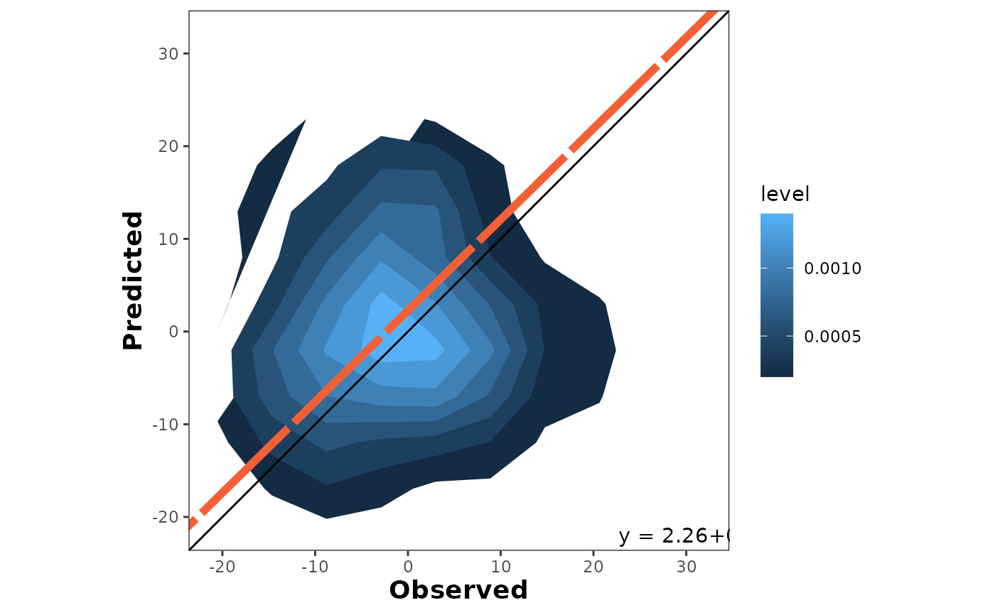
It draws a density area plot of predictions and observations with alternative axis orientation (P vs. O; O vs. P).
Usage
density_plot(
  data = NULL,
  obs,
  pred,
  n = 10,
  colors = c(low = NULL, high = NULL),
  orientation = "PO",
  print_metrics = FALSE,
  metrics_list = NULL,
  position_metrics = c(x = NULL, y = NULL),
  print_eq = TRUE,
  position_eq = c(x = NULL, y = NULL),
  eq_color = NULL,
  regline_type = NULL,
  regline_size = NULL,
  regline_color = NULL,
  na.rm = TRUE
)
Arguments
- data
(Optional) argument to call an existing data frame containing the data.
- obs
Vector with observed values (numeric).
- pred
Vector with predicted values (numeric).
- n
Argument of class numeric specifying the number of data points in each group.
- colors
Vector or list with two colors '(low, high)' to paint the density gradient.
- orientation
Argument of class string specifying the axis orientation, PO for predicted vs observed, and OP for observed vs predicted. Default is orientation = "PO".
- print_metrics
boolean TRUE/FALSE to embed metrics in the plot. Default is FALSE.
- metrics_list
vector or list of selected metrics to print on the plot.
- position_metrics
vector or list with '(x,y)' coordinates to locate the metrics_table into the plot. Default : c(x = min(obs), y = 1.05*max(pred)).
- print_eq
boolean TRUE/FALSE to embed metrics in the plot. Default is FALSE.
- position_eq
vector or list with '(x,y)' coordinates to locate the SMA equation into the plot. Default : c(x = 0.70 max(x), y = 1.25*min(y)).
- eq_color
string indicating the color of the SMA-regression text.
- regline_type
string or integer indicating the SMA-regression line-type.
- regline_size
number indicating the SMA-regression line size.
- regline_color
string indicating the SMA-regression line color.
- na.rm
Logic argument to remove rows with missing values (NA). Default is na.rm = TRUE.
Details
It creates a density plot of predicted vs. observed values. The plot also includes the 1:1 line (solid line) and the linear regression line (dashed line). By default, it places the observed on the x-axis and the predicted on the y-axis (orientation = "PO"). This can be inverted by changing the argument orientation = “OP". For more details, see online-documentation
Examples
# \donttest{
X <- rnorm(n = 100, mean = 0, sd = 10)
Y <- rnorm(n = 100, mean = 0, sd = 10)
density_plot(obs = X, pred = Y)
#> Registered S3 methods overwritten by 'ggpp':
#>   method                  from
#>   heightDetails.titleGrob ggplot2
#>   widthDetails.titleGrob  ggplot2
#> Warning: The dot-dot notation (`..level..`) was deprecated in ggplot2 3.4.0.
#> ℹ Please use `after_stat(level)` instead.
#> ℹ The deprecated feature was likely used in the metrica package.
#>   Please report the issue at
#>   <https://github.com/adriancorrendo/metrica/issues>.

# }
# }