Cate and Nelson (1971)

Description

The soiltestcorr-package also allows users to implement the quadrants analysis approach, also known as the Cate-Nelson analysis. This tutorial is intended to show how to deploy the cate_nelson_1971() function for estimating critical soil test values based on Cate and Nelson (1971). This approach is also known as the “statistical” version of the Cate-Nelson analysis. The first step of this alternative version is to estimate the CSTV (x-axis) as the minimum stv that minimizes the residual sum of squares when dividing data points in two classes (lower or greater than the CSTV) without using an arbitrary ry value. This refined version does not constrains the model performance (measured with the coefficient of determination -R2-) but the user has no control on the ry level for the CSTV estimation.

General Instructions

Load your dataframe with soil test value (stv) and relative yield (ry) data.
Specify the following arguments into the function -cate_nelson_1971()-:

(a). data (optional),

(b). stv (soil test value) and ry (relative yield) columns or vectors,

(c). plot TRUE (produces a ggplot as main output) or FALSE (DEFAULT -no plot-, only produces a list or data.frame),

(d). tidy TRUE (produces a data.frame with results) or FALSE (store results as list),

Run and check results.
Adjust plot as desired.

Tutorial

library(soiltestcorr)
#> Registered S3 methods overwritten by 'ggpp':
#>   method                  from   
#>   heightDetails.titleGrob ggplot2
#>   widthDetails.titleGrob  ggplot2

Suggested packages

# Install if needed 
library(ggplot2) # Plots
library(dplyr) # Data wrangling
library(tidyr) # Data wrangling
library(utils) # Data wrangling
library(purrr) # Mapping

This is a basic example using three different datasets:

Load datasets


# Example 1 dataset
# Fake dataset manually created
data_1 <- data.frame("RY"  = c(65,80,85,88,90,94,93,96,97,95,98,100,99,99,100),
                     "STV" = c(1,2,3,4,5,6,7,8,9,10,11,12,13,14,15))
  
# Example 2. Native fake dataset from soiltestcorr package

data_2 <- soiltestcorr::data_test


# Example 3. Native dataset from soiltestcorr package, Freitas et al.  (1966), used by Cate & Nelson (1971)
data_3 <- soiltestcorr::freitas1966

Fit cate_nelson_1971()

1. Individual fits

RY target = 90%, replace with your desired value

1.1. `tidy` = FALSE

It returns a LIST (more efficient for multiple fits at once)


# Using dataframe argument, tidy = FALSE -> return a LIST
fit_1_tidy_false <- 
  soiltestcorr::cate_nelson_1971(data = data_1,
                                 ry = RY,
                                 stv = STV,
                                 tidy = FALSE)
#> Warning in stats::chisq.test(data.frame(row.1, row.2)): Chi-squared
#> approximation may be incorrect

utils::head(fit_1_tidy_false)
#> $n
#> [1] 15
#> 
#> $CRYV
#> [1] 86.5
#> 
#> $CSTV
#> [1] 3.5
#> 
#> $R2
#> [1] 0.6942517
#> 
#> $AIC
#> [1] 97.24281
#> 
#> $BIC
#> [1] 99.36696

1.2. `tidy` = TRUE

It returns a data.frame (more organized results)


# Using dataframe argument, tidy = FALSE -> return a LIST
fit_1_tidy_true <- 
  soiltestcorr::cate_nelson_1971(data = data_1,
                                 ry = RY,
                                 stv = STV,
                                 tidy = TRUE)
#> Warning in stats::chisq.test(data.frame(row.1, row.2)): Chi-squared
#> approximation may be incorrect

utils::head(fit_1_tidy_true)
#> # A tibble: 1 × 8
#>       n  CRYV  CSTV    R2   AIC   BIC  RMSE quadrants$q.I $q.II $q.III $q.IV
#>   <int> <dbl> <dbl> <dbl> <dbl> <dbl> <dbl>         <int> <int>  <int> <int>
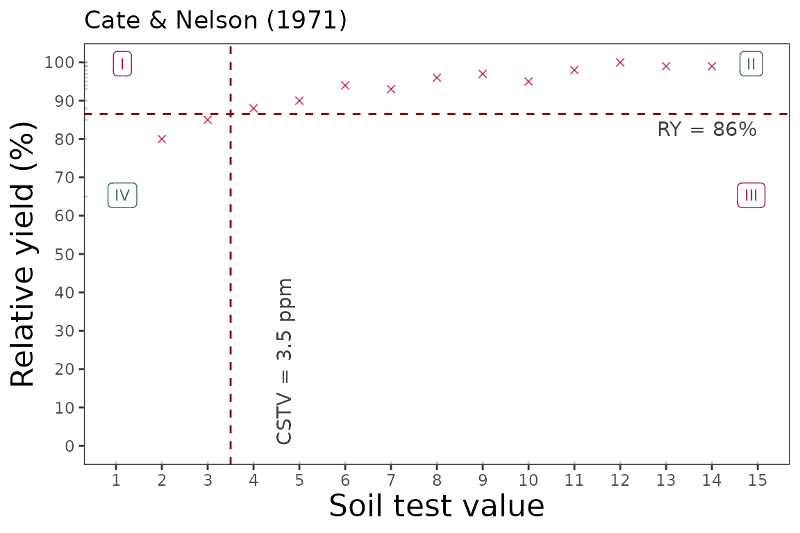
#> 1    15  86.5   3.5 0.694  97.2  99.4  5.07             0    12      0     3
#> # ℹ 2 more variables: quadrants$positive <int>, $negative <int>

1.3. Alternative using the vectors

You can call stv and ry vectors using the $.

The tidy argument still applies for controlling the output type


fit_1_vectors_list <-
  soiltestcorr::cate_nelson_1971(ry = data_1$RY,
                                 stv = data_1$STV, 
                                 tidy = FALSE)
#> Warning in stats::chisq.test(data.frame(row.1, row.2)): Chi-squared
#> approximation may be incorrect

fit_1_vectors_tidy <-
  soiltestcorr::cate_nelson_1971(ry = data_1$RY,
                                 stv = data_1$STV, 
                                 tidy = TRUE)
#> Warning in stats::chisq.test(data.frame(row.1, row.2)): Chi-squared
#> approximation may be incorrect

1.4. Data 2. Test dataset

fit_2 <-
  soiltestcorr::cate_nelson_1971(data = data_2,
                                 ry = RY,
                                 stv = STV,
                                 tidy = TRUE)

utils::head(fit_2)
#> # A tibble: 1 × 8
#>       n  CRYV  CSTV    R2   AIC   BIC  RMSE quadrants$q.I $q.II $q.III $q.IV
#>   <int> <dbl> <dbl> <dbl> <dbl> <dbl> <dbl>         <int> <int>  <int> <int>
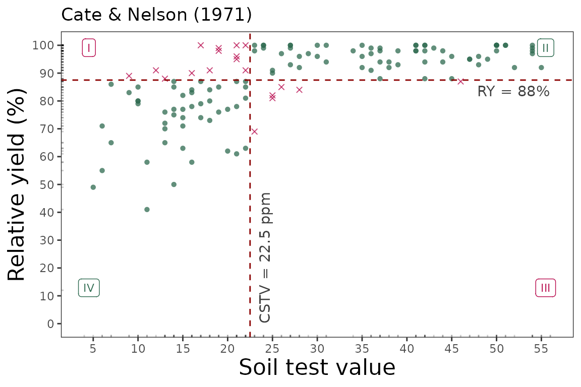
#> 1   137  87.5  22.5 0.394 1056. 1065.  11.2            13    70      6    48
#> # ℹ 2 more variables: quadrants$positive <int>, $negative <int>

1.5. Data 3. Freitas et al. 1966


fit_3 <-
  soiltestcorr::cate_nelson_1971(data = data_3,
                                 ry = RY,
                                 stv = STK,
                                 tidy = TRUE)
#> Warning in stats::chisq.test(data.frame(row.1, row.2)): Chi-squared
#> approximation may be incorrect

utils::head(fit_3)
#> # A tibble: 1 × 8
#>       n  CRYV  CSTV    R2   AIC   BIC  RMSE quadrants$q.I $q.II $q.III $q.IV
#>   <int> <dbl> <dbl> <dbl> <dbl> <dbl> <dbl>         <int> <int>  <int> <int>
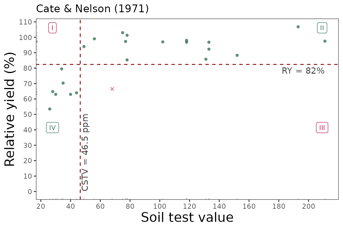
#> 1    24  82.4  46.5 0.707  183.  186.  9.64             0    15      1     8
#> # ℹ 2 more variables: quadrants$positive <int>, $negative <int>

2. Multiple fits at once

2.1. Using map

Create nested data

Note: the stv column needs to have the same name for all datasets

# 
data.all <- dplyr::bind_rows(data_1, data_2,
                      data_3 %>% dplyr::rename(STV = STK),
                     .id = "id") %>% 
  tidyr::nest(data = c("STV", "RY"))

Fit


# Run multiple examples at once with map()
fit_multiple_map <- data.all %>%
  dplyr::mutate(mod_alcc = purrr::map(data, 
                               ~ soiltestcorr::cate_nelson_1971(ry = .$RY,
                                                                stv = .$STV,
                                                                tidy = TRUE)))
#> Warning: There were 2 warnings in `dplyr::mutate()`.
#> The first warning was:
#> ℹ In argument: `mod_alcc = purrr::map(...)`.
#> Caused by warning in `stats::chisq.test()`:
#> ! Chi-squared approximation may be incorrect
#> ℹ Run `dplyr::last_dplyr_warnings()` to see the 1 remaining warning.

utils::head(fit_multiple_map)
#> # A tibble: 3 × 3
#>   id    data               mod_alcc        
#>   <chr> <list>             <list>          
#> 1 1     <tibble [15 × 2]>  <tibble [1 × 8]>
#> 2 2     <tibble [137 × 2]> <tibble [1 × 8]>
#> 3 3     <tibble [24 × 2]>  <tibble [1 × 8]>

2.2. Using group_map

Alternatively, with group_map, we do not require nested data.

However, it requires to dplyr::bind_rows and add an id column specifying the name of each dataset.

This option return models as lists objects.


fit_multiple_group_map <- 
  data.all %>% tidyr::unnest(data) %>% 
  #dplyr::bind_rows(data_1, data_2, .id = "id") %>% 
  dplyr::group_by(id) %>% 
  dplyr::group_modify(~ soiltestcorr::cate_nelson_1971(data = ., 
                                             ry = RY,
                                             stv = STV, 
                                             tidy = TRUE))
#> Warning in stats::chisq.test(data.frame(row.1, row.2)): Chi-squared
#> approximation may be incorrect
#> Warning in stats::chisq.test(data.frame(row.1, row.2)): Chi-squared
#> approximation may be incorrect

utils::head(fit_multiple_group_map)
#> # A tibble: 3 × 9
#> # Groups:   id [3]
#>   id        n  CRYV  CSTV    R2    AIC    BIC  RMSE quadrants$q.I $q.II $q.III
#>   <chr> <int> <dbl> <dbl> <dbl>  <dbl>  <dbl> <dbl>         <int> <int>  <int>
#> 1 1        15  86.5   3.5 0.694   97.2   99.4  5.07             0    12      0
#> 2 2       137  87.5  22.5 0.394 1056.  1065.  11.2             13    70      6
#> 3 3        24  82.4  46.5 0.707  183.   186.   9.64             0    15      1
#> # ℹ 3 more variables: quadrants$q.IV <int>, $positive <int>, $negative <int>

3. Bootstrapping

A suitable alternative for obtaining confidence intervals for parameters or derived quantities is bootstrapping.

Bootstrapping is a resampling technique (with replacement) that draws samples from the original data with the same size. If you have groups within your data, you can specify grouping variables as arguments in order to maintain, within each resample, the same proportion of observations than in the original dataset.

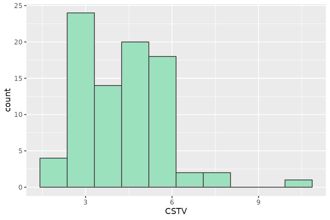
This function returns a table with as many rows as the resampling size (n) containing the results for each resample.

boot_cn71 <- soiltestcorr::boot_cn_1971(data = data_1,
                          ry = RY, stv = STV, n = 99)
#> Warning: There were 86 warnings in `dplyr::mutate()`.
#> The first warning was:
#> ℹ In argument: `model = map(...)`.
#> ℹ In group 1: `boot_id = 1`.
#> Caused by warning in `stats::chisq.test()`:
#> ! Chi-squared approximation may be incorrect
#> ℹ Run `dplyr::last_dplyr_warnings()` to see the 85 remaining warnings.

boot_cn71 %>% dplyr::slice_head(., n=5)
#> # A tibble: 5 × 9
#>   boot_id     n  CRYV  CSTV    R2   AIC   BIC  RMSE quadrants$q.I $q.II $q.III
#>     <dbl> <int> <dbl> <dbl> <dbl> <dbl> <dbl> <dbl>         <int> <int>  <int>
#> 1       1    15  95.5   8   0.859  63.8  65.9  1.66             0     8      0
#> 2       2    15  91.5   5.5 0.753  83.7  85.8  3.23             0    11      0
#> 3       3    15  91.5   5.5 0.725  80.9  83.0  2.94             0    11      0
#> 4       5    15  87.5   4   0.707  97.7  99.9  5.15             0     9      0
#> 5       7    15  87.5   4   0.687  81.8  83.9  3.03             0    13      0
#> # ℹ 3 more variables: quadrants$q.IV <int>, $positive <int>, $negative <int>

# CSTV Confidence Interval
quantile(boot_cn71$CSTV, probs = c(0.025, 0.5, 0.975))
#>   2.5%    50%  97.5% 
#> 2.0000 4.0000 7.4375

# Plot
boot_cn71 %>% 
  ggplot2::ggplot(aes(x = CSTV))+
  geom_histogram(color = "grey25", fill = "#9de0bf", bins = 10)

4. Plots

4.1. Calibration Curve

We can generate a ggplot with the same mod_alcc() function.

We just need to specify the argument plot = TRUE.


soiltestcorr::cate_nelson_1971(data = data_1, 
                       ry = RY, 
                       stv = STV, 
                       plot = TRUE)


soiltestcorr::cate_nelson_1971(data = data_2, 
                       ry = RY, 
                       stv = STV, 
                       plot = TRUE)


soiltestcorr::cate_nelson_1971(data = data_3, 
                       ry = RY, 
                       stv = STK, 
                       plot = TRUE)

References

Cate, R.B. Jr., and Nelson, L.A., 1971. A simple statistical procedure for partitioning soil test correlation data into two classes. Soil Sci. Soc. Am. Proc. 35:658-659

Adrian Correndo