Mitscherlich-type response

Description

This tutorial demonstrates the mitscherlich() function for fitting a continuous response model and estimating a critical soil test value. This function fits a Mitscherlich-type exponential regression model that follows a diminishing growth curve, and is sometimes also referred to as exponential “rise-to-the-max”. Cerrato and Blackmer (1990) expressed it as:

$y = a * (1-e^{-c(x + b)})$

where
a = asymptote,
b = model-fitting parameter ( $-b$ = X-intercept),
c = curvature parameter.

This exponential model is extensively used in agriculture to describe crops response to input since the biological meaning of its curved response. The mitscherlich() function works automatically with self-starting initial values to facilitate the model’s convergence. The mitscherlich() function allows the user to control the number of parameters, effectively constraining the response curve if theoretically justified:

type = 1, "no restriction", or "free" (DEFAULT): three parameter model; $y = a * (1-e^{-c(x + b)})$
type = 2, "asymptote 100", or "100": two parameter model where asymptote = 100% RY; $y = 100 * (1-e^{-c(x + b)})$
type = 3, "asymptote 100 from 0", or "fixed": one parameter model in which only the curvature varies and asymptote = 100 and model goes through origin; $y = 100 * (1-e^{-cx})$ .

Disadvantages this model might include:

lacks a parameter that can be directly interpreted as the critical soil test value
- the model cannot be evaluated at the asymptote as CSTV would go to Inf
- a fixed RY target for CSTV may be a somewhat arbitrary choice, but 95% is commonly used
- model may not reach 95%, for which NaN results
there is no apparent confidence interval for the derived CSTV. For this latter purpose, we recommend the user to use the boot_mitscherlich() function for a reliable confidence interval estimation of parameters and CSTV via bootstrapping (resampling with replacement).

General Instructions

Load your dataframe with soil test value (stv) and relative yield (ry) data.
Specify the following arguments into the function mitscherlich():
1. type select the type of parameterization of the model (type = 1, 2, or 3; see above)
2. data (optional)
3. stv (soil test value) and ry (relative yield) columns or vectors,
4. target (default = 95) to calculate the STV at a specific ry target.
5. tidy TRUE-default- (produces a data.frame with results) or FALSE (store results as list)
6. plot TRUE (produces a ggplot as main output) or FALSE (no plot, only results as data.frame)
7. resid TRUE (produces plots with residuals analysis) or FALSE (no plot)
Run and check results.
Check residuals plot, and warnings related to potential limitations of this model.
Adjust curve plots as desired.

Tutorial

library(soiltestcorr)
#> Registered S3 methods overwritten by 'ggpp':
#>   method                  from   
#>   heightDetails.titleGrob ggplot2
#>   widthDetails.titleGrob  ggplot2

Suggested packages

# Install if needed 
library(ggplot2) # Plots
library(dplyr) # Data wrangling
library(tidyr) # Data wrangling
library(purrr) # Mapping

Load datasets

# Native fake dataset from soiltestcorr package
corr_df <- soiltestcorr::data_test

Fit `mitscherlich()`

1. Individual fits

1.1. Different number of parameters `type = #`


# Type = 1, no restriction (3 parameters)
mitscherlich(corr_df, STV, RY, type = 1)
#> # A tibble: 1 × 13
#>   asymptote     b curvature equation  y_intercept target  CSTV   AIC  AICc   BIC
#>       <dbl> <dbl>     <dbl> <chr>           <dbl>  <dbl> <dbl> <dbl> <dbl> <dbl>
#> 1      98.0  3.91    0.0885 98(1-e^(…        28.6     95  35.5 1022. 1022. 1033.
#> # ℹ 3 more variables: R2 <dbl>, RMSE <dbl>, pvalue <dbl>
# Type = 2, fixed asymptote value at 100 (2 parameters)
mitscherlich(corr_df, STV, RY, type = 2)
#> # A tibble: 1 × 13
#>   asymptote     b curvature equation  y_intercept target  CSTV   AIC  AICc   BIC
#>       <dbl> <dbl>     <dbl> <chr>           <dbl>  <dbl> <dbl> <dbl> <dbl> <dbl>
#> 1       100  5.49    0.0763 100(1-e^…        34.2     95  33.8 1021. 1021. 1029.
#> # ℹ 3 more variables: R2 <dbl>, RMSE <dbl>, pvalue <dbl>
# Type = 3, fixed origin at 0 and asymptote at 100 (1 parameters)
mitscherlich(corr_df, STV, RY, type = 3)
#> # A tibble: 1 × 13
#>   asymptote     b curvature equation  y_intercept target  CSTV   AIC  AICc   BIC
#>       <dbl> <dbl>     <dbl> <chr>           <dbl>  <dbl> <dbl> <dbl> <dbl> <dbl>
#> 1       100     0     0.108 100(1-e^…           0     95  27.8 1031. 1032. 1037.
#> # ℹ 3 more variables: R2 <dbl>, RMSE <dbl>, pvalue <dbl>

1.2. `tidy` = FALSE

It returns a LIST (may more efficient for multiple fits at once)


# Using dataframe argument, tidy = FALSE -> return a LIST
mitscherlich(data = corr_df, STV, RY, target = 90,  tidy = FALSE)
#> $asymptote
#> [1] 97.98376
#> 
#> $b
#> [1] 3.907871
#> 
#> $curvature
#> [1] 0.08850352
#> 
#> $equation
#> [1] "98(1-e^(-0.089(x+3.9))"
#> 
#> $y_intercept
#> [1] 28.64934
#> 
#> $target
#> [1] 90
#> 
#> $CSTV
#> [1] 24.42311
#> 
#> $AIC
#> [1] 1021.64
#> 
#> $AICc
#> [1] 1021.94
#> 
#> $BIC
#> [1] 1033.32
#> 
#> $R2
#> [1] 0.54
#> 
#> $RMSE
#> [1] 9.78
#> 
#> $pvalue
#> [1] 0

1.3. Alternative using the data frame vectors

You can call stv and ry vectors using the $. The tidy argument still applies for controlling the output type.


fit_vectors_list <-mitscherlich(stv = corr_df$STV,
                                ry = corr_df$RY,
                                tidy = FALSE)

fit_vectors_tidy <-mitscherlich(stv = corr_df$STV,
                                ry = corr_df$RY,
                                tidy = TRUE)

2. Multiple fits at once

# Example 1. Fake dataset manually created
data_1 <- data.frame("RY"  = c(65,80,85,88,90,94,93,96,97,95,98,100,99,99,100),
                     "STV" = c(1,2,3,4,5,6,7,8,9,10,11,12,13,14,15))
  
# Example 2. Native fake dataset from soiltestcorr package
data_2 <- soiltestcorr::data_test


# Example 3. Native dataset from soiltestcorr package, Freitas et al.  (1966), used by Cate & Nelson (1971)
data_3 <- soiltestcorr::freitas1966 %>% 
  rename(STV = STK)

data.all <- bind_rows(data_1, data_2, data_3, .id = "id")

Note: the stv column needs to have the same name for all datasets if binding rows.

2.1. Using `map()`


# Run multiple examples at once with map()
data.all %>%
  nest(data = c("STV", "RY")) %>% 
  mutate(model = map(data, ~ mitscherlich(stv = .$STV, ry = .$RY))) %>%
  unnest(model)
#> # A tibble: 3 × 15
#>   id    data     asymptote     b curvature equation    y_intercept target   CSTV
#>   <chr> <list>       <dbl> <dbl>     <dbl> <chr>             <dbl>  <dbl>  <dbl>
#> 1 1     <tibble>      98.7  2.07    0.371  98.7(1-e^(…        52.8     95   6.77
#> 2 2     <tibble>      98.0  3.91    0.0885 98(1-e^(-0…        28.6     95  35.5 
#> 3 3     <tibble>      96.4 -8.69    0.0458 96.4(1-e^(…       -47.2     95 101.  
#> # ℹ 6 more variables: AIC <dbl>, AICc <dbl>, BIC <dbl>, R2 <dbl>, RMSE <dbl>,
#> #   pvalue <dbl>

2.2. Using `group_modify()`

Alternatively, with group_modify(), nested data is not required. However, it still requires a grouping variable (in this case, id) to identify each dataset. group_map() may also be used, though list_rbind() is required to return a tidy data frame of the model results instead of a list.


data.all %>% 
  group_by(id) %>% 
  group_modify(~ soiltestcorr::mitscherlich(data = ., STV, RY))
#> # A tibble: 3 × 14
#> # Groups:   id [3]
#>   id    asymptote     b curvature equation      y_intercept target   CSTV    AIC
#>   <chr>     <dbl> <dbl>     <dbl> <chr>               <dbl>  <dbl>  <dbl>  <dbl>
#> 1 1          98.7  2.07    0.371  98.7(1-e^(-0…        52.8     95   6.77   64.0
#> 2 2          98.0  3.91    0.0885 98(1-e^(-0.0…        28.6     95  35.5  1022. 
#> 3 3          96.4 -8.69    0.0458 96.4(1-e^(-0…       -47.2     95 101.    187. 
#> # ℹ 5 more variables: AICc <dbl>, BIC <dbl>, R2 <dbl>, RMSE <dbl>, pvalue <dbl>

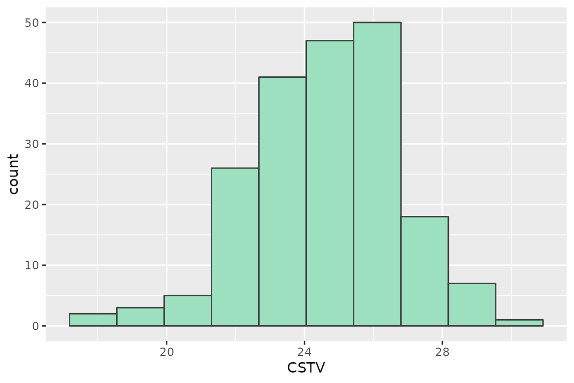
3. Bootstrapping

A suitable alternative for obtaining confidence intervals for parameters or derived quantities is bootstrapping. Bootstrapping is a resampling technique (with replacement) that draws samples from the original data with the same size. If you have groups within your data, you can specify grouping variables as arguments in order to maintain, within each resample, the same proportion of observations than in the original dataset.

This function returns a table with as many rows as the resampling size (n) containing the results for each resample.

set.seed(123)
boot_mits <- boot_mitscherlich(corr_df, STV, RY, target = 90, n = 200)
#> Warning: There were 2 warnings in `dplyr::mutate()`.
#> The first warning was:
#> ℹ In argument: `model = map(...)`.
#> ℹ In group 51: `boot_id = 51`.
#> Caused by warning in `nls.lm()`:
#> ! lmdif: info = -1. Number of iterations has reached `maxiter' == 50.
#> ℹ Run `dplyr::last_dplyr_warnings()` to see the 1 remaining warning.

boot_mits %>% head(n = 5)
#> # A tibble: 5 × 13
#>   boot_id asymptote     b curvature y_intercept target  CSTV   AIC  AICc   BIC
#>     <dbl>     <dbl> <dbl>     <dbl>       <dbl>  <dbl> <dbl> <dbl> <dbl> <dbl>
#> 1       1      98.8  2.79    0.0856        21.0     90  25.4 1029. 1029. 1041.
#> 2       2      99.0  8.28    0.0682        42.7     90  26.9 1021. 1021. 1033.
#> 3       3      98.8 10.8     0.0660        50.4     90  25.9 1007. 1008. 1019.
#> 4       4      98.9  7.01    0.0772        41.3     90  24.2  989.  989. 1001.
#> 5       5     100.  11.0     0.0630        50.3     90  24.9  986.  986.  997.
#> # ℹ 3 more variables: R2 <dbl>, RMSE <dbl>, pvalue <dbl>

# CSTV Confidence Interval
quantile(boot_mits$CSTV, probs = c(0.025, 0.5, 0.975), na.rm = TRUE)
#>     2.5%      50%    97.5% 
#> 20.22419 24.60084 28.75092

# Plot
boot_mits %>% 
  ggplot2::ggplot(aes(x = CSTV))+
  geom_histogram(color = "grey25", fill = "#9de0bf", bins = 10)

4. Plots

4.1. Calibration Curve

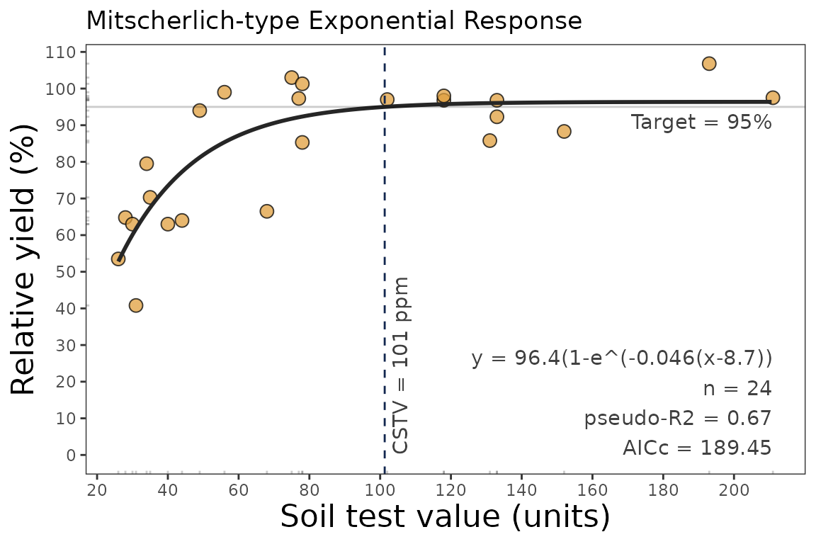
We can generate a ggplot with the same mitscherlich() function.

We just need to specify the argument plot = TRUE.

data_3 <- soiltestcorr::freitas1966

plot_mit <- mitscherlich(data_3, STK, RY, plot = TRUE)

plot_mit

4.2 Fine-tune the plots

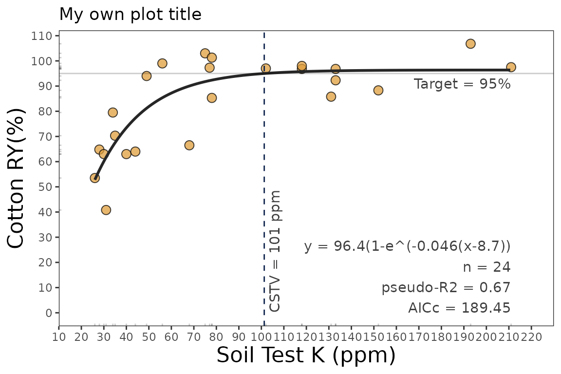
As ggplot object, plots can be adjusted in several ways, such as modifying titles and axis scales.

plot_mit +
  # Main title
  ggtitle("My own plot title")+
  # Axis titles
  labs(x = "Soil Test K (ppm)",
       y = "Cotton RY(%)") +
  # Axis scales
  scale_x_continuous(limits = c(20,220),
                     breaks = seq(0,220, by = 10))

4.3. Residuals

Set the argument resid = TRUE.


# Residuals plot
mitscherlich(data_3, STK, RY, resid = TRUE)

#> # A tibble: 1 × 13
#>   asymptote     b curvature equation  y_intercept target  CSTV   AIC  AICc   BIC
#>       <dbl> <dbl>     <dbl> <chr>           <dbl>  <dbl> <dbl> <dbl> <dbl> <dbl>
#> 1      96.4 -8.69    0.0458 96.4(1-e…       -47.2     95  101.  187.  189.  192.
#> # ℹ 3 more variables: R2 <dbl>, RMSE <dbl>, pvalue <dbl>

References

Cerrato, M. E., & Blackmer, A. M. (1990). Comparison of models for describing corn yield response to nitrogen fertilizer. Agronomy Journal, 82(1), 138–143. https://doi.org/10.2134/agronj1990.00021962008200010030x

Melsted, S.W. and Peck, T.R. (1977). The Mitscherlich-Bray Growth Function. In Soil Testing (eds T. Peck, J. Cope and D. Whitney). 10.2134/asaspecpub29.c1

Adrian Correndo & Austin Pearce