library(pacman)
p_load(agridat) # Agridat datasets
p_load(dplyr) # dplyr for data wrangling
p_load(skimr) # skimr for quick exploration of the dataTransforming Ag data with dplyr
dplyr
data wrangling
mutate
filter
select
arrange
1 Description
This lesson introduces the concept of tidy data, and a few basic data wrangling techniques using dplyr package. Today, we are using dplyr and datasets from the agridat package. If you don’t have them installed, you can do so by running:
1.1 Required packages for today
2 Why TIDY?
Well, from the hand of Tidyverse, the “tidy data” framework changed the way we code and work in R for data science. Tidy datasets are easy to manipulate, model and visualize, and have a specific structure (Wickham 2014):
Each variable is a column,
Each observation is a row, and
Each value have its own cell.
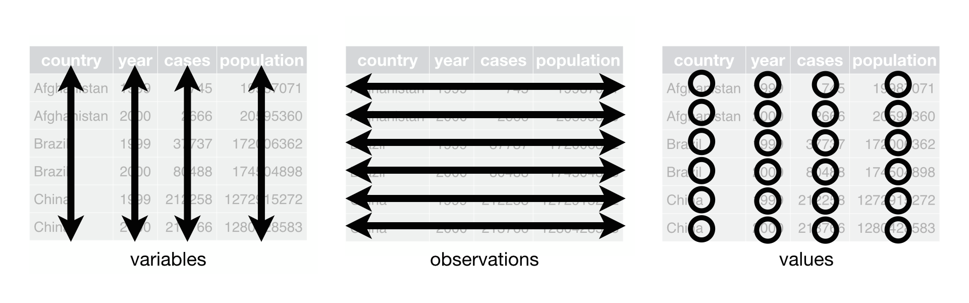 Tidy-data structure. Following three rules makes a dataset tidy: variables are in columns, observations are in rows, and values are in cells. Source: (Wickham and Grolemund 2017).
Example of tidy data:
# Example of tidy data
tidy_data <- data.frame(
  subject = c(1, 2, 3),
  gender = c("M", "F", "F"),
  score = c(90, 95, 88)
)

tidy_data
subject gender score
1 1 M 90
2 2 F 95
3 3 F 882.0.1 Free HTML books
2.1 What is a Data Frame?
A data frame is a two-dimensional table-like structure in R, where columns can contain different types of data (e.g., numeric, character). It is the default structure for datasets loaded from CSV files or data packages.
2.1.1 open a data frame
# Load the wheat dataset from agricolae (which is a data frame)
wheat_data <- agridat::payne.wheat

# Check the structure of the data frame
str(wheat_data)
'data.frame': 480 obs. of 4 variables:
$ rotation: Factor w/ 6 levels "AB","AF","Lc3",..: 1 1 1 1 2 2 2 2 5 5 ...
$ nitro : int 0 70 140 210 0 70 140 210 0 70 ...
$ year : int 1981 1981 1981 1981 1981 1981 1981 1981 1981 1981 ...
$ yield : num 3.84 6.59 7.49 7.39 3.06 6.32 7.61 7.78 5.82 7.52 ...2.2 What is a Tibble?
A tibble is a modern version of a data frame, introduced by the tibble package. It offers several improvements:
•   Tibbles don’t convert characters to factors by default.
•   Printing is more concise and doesn’t overwhelm you with too much data.
•   Tibbles are more explicit with column types when printed.
2.2.1 create a tibble
# Convert the wheat data frame to a tibble
wheat_tibble <- as_tibble(wheat_data)

# Check the structure of the tibble
wheat_tibble
# A tibble: 480 × 4
rotation nitro year yield
<fct> <int> <int> <dbl>
1 AB 0 1981 3.84
2 AB 70 1981 6.59
3 AB 140 1981 7.49
4 AB 210 1981 7.39
5 AF 0 1981 3.06
6 AF 70 1981 6.32
7 AF 140 1981 7.61
8 AF 210 1981 7.78
9 Ln3 0 1981 5.82
10 Ln3 70 1981 7.52
# ℹ 470 more rows2.3 iii. Key Differences between Data Frames and Tibbles
1. **Printing**:• Data Frames print the entire dataset unless you limit the number of rows. No information about column types is displayed. • Tibbles print only the first 10 rows and automatically show column types.
2.3.1 Example:
# Print the entire data frame
print(wheat_data)
rotation nitro year yield
1 AB 0 1981 3.84
2 AB 70 1981 6.59
3 AB 140 1981 7.49
4 AB 210 1981 7.39
5 AF 0 1981 3.06
6 AF 70 1981 6.32
7 AF 140 1981 7.61
8 AF 210 1981 7.78
9 Ln3 0 1981 5.82
10 Ln3 70 1981 7.52
11 Ln3 140 1981 8.12
12 Ln3 210 1981 7.40
13 Ln8 0 1981 4.71
14 Ln8 70 1981 6.52
15 Ln8 140 1981 8.03
16 Ln8 210 1981 7.83
17 Lc3 0 1981 5.35
18 Lc3 70 1981 6.70
19 Lc3 140 1981 7.69
20 Lc3 210 1981 7.53
21 Lc8 0 1981 6.47
22 Lc8 70 1981 7.84
23 Lc8 140 1981 7.98
24 Lc8 210 1981 7.68
25 AB 0 1982 4.47
26 AB 70 1982 6.38
27 AB 140 1982 7.82
28 AB 210 1982 8.13
29 AF 0 1982 4.30
30 AF 70 1982 6.82
31 AF 140 1982 8.16
32 AF 210 1982 8.52
33 Ln3 0 1982 5.37
34 Ln3 70 1982 7.91
35 Ln3 140 1982 7.53
36 Ln3 210 1982 8.46
37 Ln8 0 1982 5.55
38 Ln8 70 1982 8.04
39 Ln8 140 1982 8.27
40 Ln8 210 1982 7.31
41 Lc3 0 1982 5.16
42 Lc3 70 1982 7.81
43 Lc3 140 1982 8.38
44 Lc3 210 1982 7.40
45 Lc8 0 1982 6.56
46 Lc8 70 1982 8.36
47 Lc8 140 1982 8.60
48 Lc8 210 1982 8.41
49 AB 0 1983 4.11
50 AB 70 1983 6.28
51 AB 140 1983 8.70
52 AB 210 1983 8.17
53 AF 0 1983 3.76
54 AF 70 1983 6.79
55 AF 140 1983 8.50
56 AF 210 1983 9.43
57 Ln3 0 1983 3.86
58 Ln3 70 1983 7.05
59 Ln3 140 1983 8.06
60 Ln3 210 1983 8.28
61 Ln8 0 1983 4.45
62 Ln8 70 1983 7.23
63 Ln8 140 1983 7.48
64 Ln8 210 1983 6.93
65 Lc3 0 1983 6.36
66 Lc3 70 1983 9.67
67 Lc3 140 1983 9.34
68 Lc3 210 1983 8.40
69 Lc8 0 1983 7.39
70 Lc8 70 1983 9.64
71 Lc8 140 1983 8.80
72 Lc8 210 1983 8.66
73 AB 0 1984 3.66
74 AB 70 1984 6.56
75 AB 140 1984 7.74
76 AB 210 1984 9.41
77 AF 0 1984 4.28
78 AF 70 1984 8.94
79 AF 140 1984 9.12
80 AF 210 1984 9.35
81 Ln3 0 1984 4.92
82 Ln3 70 1984 7.66
83 Ln3 140 1984 9.75
84 Ln3 210 1984 10.35
85 Ln8 0 1984 5.46
86 Ln8 70 1984 8.68
87 Ln8 140 1984 9.20
88 Ln8 210 1984 10.33
89 Lc3 0 1984 7.18
90 Lc3 70 1984 11.06
91 Lc3 140 1984 10.52
92 Lc3 210 1984 9.88
93 Lc8 0 1984 7.51
94 Lc8 70 1984 9.66
95 Lc8 140 1984 11.04
96 Lc8 210 1984 9.36
97 AB 0 1985 2.39
98 AB 70 1985 5.90
99 AB 140 1985 7.76
100 AB 210 1985 8.62
101 AF 0 1985 2.03
102 AF 70 1985 5.46
103 AF 140 1985 7.72
104 AF 210 1985 9.20
105 Ln3 0 1985 4.24
106 Ln3 70 1985 7.26
107 Ln3 140 1985 8.26
108 Ln3 210 1985 9.69
109 Ln8 0 1985 4.07
110 Ln8 70 1985 6.98
111 Ln8 140 1985 8.39
112 Ln8 210 1985 8.55
113 Lc3 0 1985 4.97
114 Lc3 70 1985 7.64
115 Lc3 140 1985 9.57
116 Lc3 210 1985 8.84
117 Lc8 0 1985 4.44
118 Lc8 70 1985 8.08
119 Lc8 140 1985 8.76
120 Lc8 210 1985 10.19
121 AB 0 1986 4.17
122 AB 70 1986 6.91
123 AB 140 1986 7.21
124 AB 210 1986 8.53
125 AF 0 1986 4.08
126 AF 70 1986 5.08
127 AF 140 1986 6.32
128 AF 210 1986 7.88
129 Ln3 0 1986 3.36
130 Ln3 70 1986 5.65
131 Ln3 140 1986 6.62
132 Ln3 210 1986 6.05
133 Ln8 0 1986 4.68
134 Ln8 70 1986 6.55
135 Ln8 140 1986 7.20
136 Ln8 210 1986 6.84
137 Lc3 0 1986 6.14
138 Lc3 70 1986 7.15
139 Lc3 140 1986 6.89
140 Lc3 210 1986 6.20
141 Lc8 0 1986 6.09
142 Lc8 70 1986 7.31
143 Lc8 140 1986 6.85
144 Lc8 210 1986 6.75
145 AB 0 1987 4.39
146 AB 70 1987 6.18
147 AB 140 1987 6.75
148 AB 210 1987 7.84
149 AF 0 1987 3.02
150 AF 70 1987 5.56
151 AF 140 1987 6.60
152 AF 210 1987 6.43
153 Ln3 0 1987 4.41
154 Ln3 70 1987 6.55
155 Ln3 140 1987 7.59
156 Ln3 210 1987 7.13
157 Ln8 0 1987 4.80
158 Ln8 70 1987 6.74
159 Ln8 140 1987 7.86
160 Ln8 210 1987 7.00
161 Lc3 0 1987 5.51
162 Lc3 70 1987 7.24
163 Lc3 140 1987 7.74
164 Lc3 210 1987 7.61
165 Lc8 0 1987 5.26
166 Lc8 70 1987 7.48
167 Lc8 140 1987 8.31
168 Lc8 210 1987 8.13
169 AB 0 1988 2.98
170 AB 70 1988 6.28
171 AB 140 1988 6.77
172 AB 210 1988 6.20
173 AF 0 1988 3.09
174 AF 70 1988 6.60
175 AF 140 1988 6.63
176 AF 210 1988 6.61
177 Ln3 0 1988 4.01
178 Ln3 70 1988 6.77
179 Ln3 140 1988 7.12
180 Ln3 210 1988 6.14
181 Ln8 0 1988 4.34
182 Ln8 70 1988 6.73
183 Ln8 140 1988 7.46
184 Ln8 210 1988 7.23
185 Lc3 0 1988 5.68
186 Lc3 70 1988 7.39
187 Lc3 140 1988 7.54
188 Lc3 210 1988 7.51
189 Lc8 0 1988 5.26
190 Lc8 70 1988 7.87
191 Lc8 140 1988 6.94
192 Lc8 210 1988 7.06
193 AB 0 1989 1.16
194 AB 70 1989 3.94
195 AB 140 1989 4.58
196 AB 210 1989 4.74
197 AF 0 1989 2.80
198 AF 70 1989 4.92
199 AF 140 1989 5.17
200 AF 210 1989 5.82
201 Ln3 0 1989 4.04
202 Ln3 70 1989 5.94
203 Ln3 140 1989 6.10
204 Ln3 210 1989 6.04
205 Ln8 0 1989 3.77
206 Ln8 70 1989 5.58
207 Ln8 140 1989 5.56
208 Ln8 210 1989 4.91
209 Lc3 0 1989 5.45
210 Lc3 70 1989 6.28
211 Lc3 140 1989 6.12
212 Lc3 210 1989 5.81
213 Lc8 0 1989 4.91
214 Lc8 70 1989 6.69
215 Lc8 140 1989 6.39
216 Lc8 210 1989 5.06
217 AB 0 1990 1.47
218 AB 70 1990 4.94
219 AB 140 1990 5.83
220 AB 210 1990 6.33
221 AF 0 1990 1.38
222 AF 70 1990 5.72
223 AF 140 1990 6.30
224 AF 210 1990 5.18
225 Ln3 0 1990 1.73
226 Ln3 70 1990 4.94
227 Ln3 140 1990 5.43
228 Ln3 210 1990 6.17
229 Ln8 0 1990 2.62
230 Ln8 70 1990 5.79
231 Ln8 140 1990 5.08
232 Ln8 210 1990 5.25
233 Lc3 0 1990 3.59
234 Lc3 70 1990 6.06
235 Lc3 140 1990 7.20
236 Lc3 210 1990 6.42
237 Lc8 0 1990 3.31
238 Lc8 70 1990 6.51
239 Lc8 140 1990 6.65
240 Lc8 210 1990 6.99
241 AB 0 1991 4.48
242 AB 70 1991 8.56
243 AB 140 1991 9.94
244 AB 210 1991 10.23
245 AF 0 1991 3.46
246 AF 70 1991 8.00
247 AF 140 1991 9.75
248 AF 210 1991 10.57
249 Ln3 0 1991 6.75
250 Ln3 70 1991 8.85
251 Ln3 140 1991 9.96
252 Ln3 210 1991 10.41
253 Ln8 0 1991 5.94
254 Ln8 70 1991 8.83
255 Ln8 140 1991 9.64
256 Ln8 210 1991 9.75
257 Lc3 0 1991 6.47
258 Lc3 70 1991 9.37
259 Lc3 140 1991 10.46
260 Lc3 210 1991 10.48
261 Lc8 0 1991 6.08
262 Lc8 70 1991 8.81
263 Lc8 140 1991 9.63
264 Lc8 210 1991 10.10
265 AB 0 1992 6.31
266 AB 70 1992 7.84
267 AB 140 1992 7.21
268 AB 210 1992 6.81
269 AF 0 1992 3.82
270 AF 70 1992 8.05
271 AF 140 1992 8.21
272 AF 210 1992 7.59
273 Ln3 0 1992 2.73
274 Ln3 70 1992 6.47
275 Ln3 140 1992 7.49
276 Ln3 210 1992 7.26
277 Ln8 0 1992 4.19
278 Ln8 70 1992 7.17
279 Ln8 140 1992 7.54
280 Ln8 210 1992 6.67
281 Lc3 0 1992 6.33
282 Lc3 70 1992 7.48
283 Lc3 140 1992 6.13
284 Lc3 210 1992 4.79
285 Lc8 0 1992 7.11
286 Lc8 70 1992 6.65
287 Lc8 140 1992 6.45
288 Lc8 210 1992 6.14
289 AB 0 1993 3.11
290 AB 70 1993 5.92
291 AB 140 1993 5.89
292 AB 210 1993 6.63
293 AF 0 1993 2.86
294 AF 70 1993 5.79
295 AF 140 1993 6.72
296 AF 210 1993 7.37
297 Ln3 0 1993 3.13
298 Ln3 70 1993 5.40
299 Ln3 140 1993 6.60
300 Ln3 210 1993 6.52
301 Ln8 0 1993 3.42
302 Ln8 70 1993 5.16
303 Ln8 140 1993 6.47
304 Ln8 210 1993 6.55
305 Lc3 0 1993 5.58
306 Lc3 70 1993 7.01
307 Lc3 140 1993 7.69
308 Lc3 210 1993 7.91
309 Lc8 0 1993 6.08
310 Lc8 70 1993 7.03
311 Lc8 140 1993 7.20
312 Lc8 210 1993 7.69
313 AB 0 1994 0.93
314 AB 70 1994 3.94
315 AB 140 1994 4.04
316 AB 210 1994 3.51
317 AF 0 1994 1.80
318 AF 70 1994 5.32
319 AF 140 1994 8.08
320 AF 210 1994 8.55
321 Ln3 0 1994 4.76
322 Ln3 70 1994 6.16
323 Ln3 140 1994 7.35
324 Ln3 210 1994 7.14
325 Ln8 0 1994 3.64
326 Ln8 70 1994 5.14
327 Ln8 140 1994 7.00
328 Ln8 210 1994 7.16
329 Lc3 0 1994 5.06
330 Lc3 70 1994 6.00
331 Lc3 140 1994 6.28
332 Lc3 210 1994 7.50
333 Lc8 0 1994 3.46
334 Lc8 70 1994 6.48
335 Lc8 140 1994 6.07
336 Lc8 210 1994 7.53
337 AB 0 1995 1.30
338 AB 70 1995 4.21
339 AB 140 1995 4.35
340 AB 210 1995 4.35
341 AF 0 1995 1.27
342 AF 70 1995 3.82
343 AF 140 1995 4.60
344 AF 210 1995 4.96
345 Ln3 0 1995 2.17
346 Ln3 70 1995 5.01
347 Ln3 140 1995 5.39
348 Ln3 210 1995 5.79
349 Ln8 0 1995 2.52
350 Ln8 70 1995 5.71
351 Ln8 140 1995 5.36
352 Ln8 210 1995 6.53
353 Lc3 0 1995 2.57
354 Lc3 70 1995 5.70
355 Lc3 140 1995 6.46
356 Lc3 210 1995 5.78
357 Lc8 0 1995 3.52
358 Lc8 70 1995 6.60
359 Lc8 140 1995 6.36
360 Lc8 210 1995 6.14
361 AB 0 1996 1.19
362 AB 70 1996 7.24
363 AB 140 1996 7.80
364 AB 210 1996 8.43
365 AF 0 1996 0.65
366 AF 70 1996 6.60
367 AF 140 1996 7.69
368 AF 210 1996 7.79
369 Ln3 0 1996 3.82
370 Ln3 70 1996 7.19
371 Ln3 140 1996 7.15
372 Ln3 210 1996 8.41
373 Ln8 0 1996 6.37
374 Ln8 70 1996 8.23
375 Ln8 140 1996 8.77
376 Ln8 210 1996 8.46
377 Lc3 0 1996 5.23
378 Lc3 70 1996 7.76
379 Lc3 140 1996 8.19
380 Lc3 210 1996 8.67
381 Lc8 0 1996 5.73
382 Lc8 70 1996 7.97
383 Lc8 140 1996 8.48
384 Lc8 210 1996 8.28
385 AB 0 1997 1.58
386 AB 70 1997 5.73
387 AB 140 1997 7.37
388 AB 210 1997 7.88
389 AF 0 1997 2.40
390 AF 70 1997 6.52
391 AF 140 1997 9.25
392 AF 210 1997 9.24
393 Ln3 0 1997 1.74
394 Ln3 70 1997 3.83
395 Ln3 140 1997 5.15
396 Ln3 210 1997 5.02
397 Ln8 0 1997 2.53
398 Ln8 70 1997 6.20
399 Ln8 140 1997 6.93
400 Ln8 210 1997 7.25
401 Lc3 0 1997 4.40
402 Lc3 70 1997 7.70
403 Lc3 140 1997 8.01
404 Lc3 210 1997 8.30
405 Lc8 0 1997 4.10
406 Lc8 70 1997 6.78
407 Lc8 140 1997 7.36
408 Lc8 210 1997 7.43
409 AB 0 1998 3.21
410 AB 70 1998 6.70
411 AB 140 1998 9.35
412 AB 210 1998 10.26
413 AF 0 1998 2.52
414 AF 70 1998 6.35
415 AF 140 1998 8.80
416 AF 210 1998 9.72
417 Ln3 0 1998 3.77
418 Ln3 70 1998 7.13
419 Ln3 140 1998 8.67
420 Ln3 210 1998 9.62
421 Ln8 0 1998 4.97
422 Ln8 70 1998 7.77
423 Ln8 140 1998 9.21
424 Ln8 210 1998 9.24
425 Lc3 0 1998 4.78
426 Lc3 70 1998 7.48
427 Lc3 140 1998 8.50
428 Lc3 210 1998 8.75
429 Lc8 0 1998 4.11
430 Lc8 70 1998 7.55
431 Lc8 140 1998 9.01
432 Lc8 210 1998 8.98
433 AB 0 1999 0.00
434 AB 70 1999 1.97
435 AB 140 1999 3.44
436 AB 210 1999 2.28
437 AF 0 1999 0.52
438 AF 70 1999 6.55
439 AF 140 1999 7.53
440 AF 210 1999 8.48
441 Ln3 0 1999 1.69
442 Ln3 70 1999 6.58
443 Ln3 140 1999 7.58
444 Ln3 210 1999 7.83
445 Ln8 0 1999 3.42
446 Ln8 70 1999 6.59
447 Ln8 140 1999 8.26
448 Ln8 210 1999 6.51
449 Lc3 0 1999 4.42
450 Lc3 70 1999 7.27
451 Lc3 140 1999 8.65
452 Lc3 210 1999 9.54
453 Lc8 0 1999 1.79
454 Lc8 70 1999 4.65
455 Lc8 140 1999 5.54
456 Lc8 210 1999 4.95
457 AB 0 2000 1.45
458 AB 70 2000 4.54
459 AB 140 2000 4.52
460 AB 210 2000 5.53
461 AF 0 2000 0.96
462 AF 70 2000 4.87
463 AF 140 2000 6.28
464 AF 210 2000 7.39
465 Ln3 0 2000 3.40
466 Ln3 70 2000 7.06
467 Ln3 140 2000 8.64
468 Ln3 210 2000 8.71
469 Ln8 0 2000 3.42
470 Ln8 70 2000 6.58
471 Ln8 140 2000 7.22
472 Ln8 210 2000 7.49
473 Lc3 0 2000 5.05
474 Lc3 70 2000 8.24
475 Lc3 140 2000 8.96
476 Lc3 210 2000 10.33
477 Lc8 0 2000 4.31
478 Lc8 70 2000 7.47
479 Lc8 140 2000 8.95
480 Lc8 210 2000 9.65# Print the tibble (shows only first 10 rows and column types)
print(wheat_tibble)# A tibble: 480 × 4
rotation nitro year yield
<fct> <int> <int> <dbl>
1 AB 0 1981 3.84
2 AB 70 1981 6.59
3 AB 140 1981 7.49
4 AB 210 1981 7.39
5 AF 0 1981 3.06
6 AF 70 1981 6.32
7 AF 140 1981 7.61
8 AF 210 1981 7.78
9 Ln3 0 1981 5.82
10 Ln3 70 1981 7.52
# ℹ 470 more rows3 A package for data manipulation…🚀
![]()
The dplyr package in R provides powerful tools for transforming and analyzing data. In this tutorial, we’ll use an agricultural dataset to explore some common dplyr functions like filter(), mutate(), summarize(), and group_by().
3.1 Why using R Packages? 💡
- Efficiency: Avoid rewriting code for common tasks.
- Consistency: Standardized code structure and naming conventions.
- Reproducibility: Ensures that your work is easier to share and reproduce.
- Intuitive: R packages use functions with intuitive names of functions, so you can spend less time learning the code & more time learning to solve practical problems.
3.2 Example 1: mutate()
Packages like dplyr simplify tasks by providing clean, concise code for data manipulation.
1. Create a new column: total, which is the sum of two existing columns (var1 and var2).
3.2.0.1 Base R version
# Sample data
df <- data.frame(var1 = c(1, 2, 3), var2 = c(4, 5, 6))

# Adding a new column using base R
df$total <- df$var1 + df$var2
3.2.0.2 dplyr package (Tidyverse)
library(dplyr)

# Using mutate to add a new column
df <- df %>%
  mutate(total = var1 + var2)
3.3 Example 2: filter()
2. Filtering: get values of var1 greater than 2.
3.3.0.1 Base R version
# Filter rows using base R
filtered_df <- df[df$var1 > 2, ]
3.3.0.2 dplyr package (Tidyverse)
# Filter rows using dplyr
filtered_df <- filter(data = df, var1 > 2)
3.4 Example 3: select()
3. Select specific variables: get var1 and var3.
3.4.0.1 Base R version
# Select columns using base R
selected_df <- df[ , c("var1","var3")]
3.4.0.2 dplyr package (Tidyverse)
# Filter rows using dplyr
filtered_df <- select(data = df, var1, var3)
4 Corn Dataset:
For this tutorial, we’ll use the lasrosas.corn dataset from the ‘agridat’ package, which contains information on corn varieties, yields, and topographical features. First, let’s load the required packages and inspect the dataset: ## Read data
# Load dataset
data("lasrosas.corn") # This creates an object with the name of the dataset "lasrosas.corn"

# Store the data with another name
corn_data <- lasrosas.corn
4.1 Inspect data
4.1.1 glimpse
The glimpse() function provides an overview of the dataset, including variable names and data types.
# Inspect the dataset
glimpse(corn_data)
Rows: 3,443
Columns: 9
$ year <int> 1999, 1999, 1999, 1999, 1999, 1999, 1999, 1999, 1999, 1999, 1999…
$ lat <dbl> -33.05113, -33.05115, -33.05116, -33.05117, -33.05118, -33.05120…
$ long <dbl> -63.84886, -63.84879, -63.84872, -63.84865, -63.84858, -63.84851…
$ yield <dbl> 72.14, 73.79, 77.25, 76.35, 75.55, 70.24, 76.17, 69.17, 69.77, 6…
$ nitro <dbl> 131.5, 131.5, 131.5, 131.5, 131.5, 131.5, 131.5, 131.5, 131.5, 1…
$ topo <fct> W, W, W, W, W, W, W, W, W, W, W, W, W, W, W, W, W, W, W, W, W, W…
$ bv <dbl> 162.60, 170.49, 168.39, 176.68, 171.46, 170.56, 172.94, 171.86, …
$ rep <fct> R1, R1, R1, R1, R1, R1, R1, R1, R1, R1, R1, R1, R1, R1, R1, R1, …
$ nf <fct> N5, N5, N5, N5, N5, N5, N5, N5, N5, N5, N5, N5, N5, N5, N5, N5, …4.1.2 skim
The skim() function from the ‘skimr’ allows to take a deeper look to all the variables (columns), creating a quick summary that reports the presence of missing values, etc., etc.
skimr::skim(corn_data)| Name | corn_data |
| Number of rows | 3443 |
| Number of columns | 9 |
| _______________________ | |
| Column type frequency: | |
| factor | 3 |
| numeric | 6 |
| ________________________ | |
| Group variables | None |
Variable type: factor
| skim_variable | n_missing | complete_rate | ordered | n_unique | top_counts |
|---|---|---|---|---|---|
| topo | 0 | 1 | FALSE | 4 | W: 1043, LO: 885, HT: 785, E: 730 |
| rep | 0 | 1 | FALSE | 3 | R3: 1149, R1: 1147, R2: 1147 |
| nf | 0 | 1 | FALSE | 6 | N1: 577, N3: 575, N5: 575, N0: 573 |
Variable type: numeric
| skim_variable | n_missing | complete_rate | mean | sd | p0 | p25 | p50 | p75 | p100 | hist |
|---|---|---|---|---|---|---|---|---|---|---|
| year | 0 | 1 | 1999.99 | 1.00 | 1999.00 | 1999.00 | 1999.00 | 2001.00 | 2001.00 | ▇▁▁▁▇ |
| lat | 0 | 1 | -33.05 | 0.00 | -33.05 | -33.05 | -33.05 | -33.05 | -33.05 | ▃▇▆▃▁ |
| long | 0 | 1 | -63.85 | 0.00 | -63.85 | -63.85 | -63.85 | -63.84 | -63.84 | ▇▇▇▇▇ |
| yield | 0 | 1 | 69.83 | 19.83 | 12.66 | 54.54 | 66.63 | 84.68 | 117.90 | ▁▅▇▃▃ |
| nitro | 0 | 1 | 64.57 | 42.60 | 0.00 | 29.00 | 66.00 | 106.00 | 131.50 | ▅▇▇▂▇ |
| bv | 0 | 1 | 174.42 | 9.68 | 91.74 | 168.48 | 173.08 | 179.39 | 213.82 | ▁▁▁▇▁ |
4.2 Adding New Variables with mutate()
You can add new columns to your dataset with mutate(). Let’s calculate the yield in tons per hectare (assuming the current yield is in kilograms):
# Add a column for yield in tons
corn_data <- corn_data %>%
  # New column, `yield_tons`, with the transformed yield values.
  mutate(yield_tons = yield / 1000)

head(corn_data)
year lat long yield nitro topo bv rep nf yield_tons
1 1999 -33.05113 -63.84886 72.14 131.5 W 162.60 R1 N5 0.07214
2 1999 -33.05115 -63.84879 73.79 131.5 W 170.49 R1 N5 0.07379
3 1999 -33.05116 -63.84872 77.25 131.5 W 168.39 R1 N5 0.07725
4 1999 -33.05117 -63.84865 76.35 131.5 W 176.68 R1 N5 0.07635
5 1999 -33.05118 -63.84858 75.55 131.5 W 171.46 R1 N5 0.07555
6 1999 -33.05120 -63.84851 70.24 131.5 W 170.56 R1 N5 0.070244.3 Filtering Data
To focus on specific data, we can use filter(). For example, let’s filter the data to include only rows where the nitrogen applied (nitro) is greater than 100:
# Filter rows with nitro > 100
high_nitro <- corn_data %>%
  # only rows where the `nitro` column has values greater than 100.
  filter(nitro > 100)

head(high_nitro)
year lat long yield nitro topo bv rep nf yield_tons
1 1999 -33.05113 -63.84886 72.14 131.5 W 162.60 R1 N5 0.07214
2 1999 -33.05115 -63.84879 73.79 131.5 W 170.49 R1 N5 0.07379
3 1999 -33.05116 -63.84872 77.25 131.5 W 168.39 R1 N5 0.07725
4 1999 -33.05117 -63.84865 76.35 131.5 W 176.68 R1 N5 0.07635
5 1999 -33.05118 -63.84858 75.55 131.5 W 171.46 R1 N5 0.07555
6 1999 -33.05120 -63.84851 70.24 131.5 W 170.56 R1 N5 0.070244.4 Selecting columns
To select specific variables, we use select(), which selects specific columns from the dataset.
# Select specific columns
selected_data <- corn_data %>% select(yield, nitro, topo)
head(selected_data)
yield nitro topo
1 72.14 131.5 W
2 73.79 131.5 W
3 77.25 131.5 W
4 76.35 131.5 W
5 75.55 131.5 W
6 70.24 131.5 W4.5 Renaming columns
When we need to change names of columns, we can use rename():
# Rename a column
renamed_data <- corn_data %>% rename(Nitrogen = nitro)
head(renamed_data)
year lat long yield Nitrogen topo bv rep nf yield_tons
1 1999 -33.05113 -63.84886 72.14 131.5 W 162.60 R1 N5 0.07214
2 1999 -33.05115 -63.84879 73.79 131.5 W 170.49 R1 N5 0.07379
3 1999 -33.05116 -63.84872 77.25 131.5 W 168.39 R1 N5 0.07725
4 1999 -33.05117 -63.84865 76.35 131.5 W 176.68 R1 N5 0.07635
5 1999 -33.05118 -63.84858 75.55 131.5 W 171.46 R1 N5 0.07555
6 1999 -33.05120 -63.84851 70.24 131.5 W 170.56 R1 N5 0.070244.6 Arranging data
To reorder the data based on specific criteria, we can use arrange(), which will arrange rows by a variable in ascending or descending order.
# Arrange data by yield in descending order
arranged_data <- corn_data %>% arrange(desc(yield))
head(arranged_data)
year lat long yield nitro topo bv rep nf yield_tons
1 2001 -33.05086 -63.84317 117.90 99.8 LO 162.17 R3 N4 0.11790
2 2001 -33.05125 -63.84245 117.19 124.6 LO 165.81 R3 N5 0.11719
3 2001 -33.05181 -63.84323 116.64 124.6 LO 159.75 R1 N5 0.11664
4 2001 -33.05084 -63.84324 114.94 99.8 LO 166.27 R3 N4 0.11494
5 2001 -33.05134 -63.84299 114.46 99.8 LO 164.58 R2 N4 0.11446
6 2001 -33.05127 -63.84238 114.08 124.6 LO 170.94 R3 N5 0.114084.7 Finding unique values
To find out what are the unique values of a variable, we can use distinct(), which will return the unique values within a column.
# Unique values in topo
unique_topo <- corn_data %>% distinct(topo)
unique_topo
topo
1 W
2 HT
3 E
4 LO4.8 Counting
The function count() counts the number of observations within a group.
# Count observations by topo
topo_count <- corn_data %>% count(topo)
topo_count
topo n
1 E 730
2 HT 785
3 LO 885
4 W 10434.9 Summarizing Data
To get a quick overview of your data, you can use summarize() in combination with group_by(). For example, let’s calculate the average yield for each topographical category (topo):
# Average yield by topography
average_yield_topo <- corn_data %>%
  group_by(topo) %>%
  summarize(avg_yield = mean(yield, na.rm = TRUE))
average_yield_topo
# A tibble: 4 × 2
topo avg_yield
<fct> <dbl>
1 E 78.7
2 HT 48.6
3 LO 84.9
4 W 66.8# Average yield by year and topography
average_yield_topoyear <- corn_data %>%
group_by(year, topo) %>%
summarize(avg_yield = mean(yield, na.rm = TRUE))`summarise()` has grouped output by 'year'. You can override using the
`.groups` argument.average_yield_topoyear# A tibble: 8 × 3
# Groups: year [2]
year topo avg_yield
<int> <fct> <dbl>
1 1999 E 64.8
2 1999 HT 53.4
3 1999 LO 71.2
4 1999 W 66.0
5 2001 E 92.7
6 2001 HT 44.7
7 2001 LO 99.9
8 2001 W 67.7This groups the data by topo and calculates the mean yield for each group.
5 Hands-On Exercise
Try the following tasks using the lasrosas.corn dataset:
- Filter the data to include only rows where the yield is greater than 6000.
- Add a new column that calculates yield per kilogram of nitrogen applied.
- Summarize the data to find the total yield for each
topocategory. - Arrange the data by
nitroin ascending order. - Use
select()to create a dataset with only theyield,topo, andnitrocolumns.
Submit your code and results to the class discussion forum. Happy coding!
6 Conclusion
The dplyr package simplifies data transformation and analysis tasks, making it easier to work with agricultural datasets like the one in this tutorial. Use these functions and try the hands-on exercise to deepen your understanding.
Happy coding!
References
Wickham, Hadley. 2014. “Tidy Data.” Journal of Statistical Software 59 (10). https://doi.org/10.18637/jss.v059.i10.
Wickham, Hadley, and Garrett Grolemund. 2017. R for Data Science: Import, Tidy, Transform, Visualize, and Model Data. 1st ed. Paperback; O’Reilly Media. http://r4ds.had.co.nz/.