Iteration in R: The Power of `purrr`

iteration

purrr

functional programming

case study

Author

Dr. Adrian Correndo

Published

February 11, 2026

Description

This lesson explores iteration in R, focusing on the power of the purrr package for functional programming. We’ll compare traditional for loops with purrr’s map() functions to illustrate more efficient and readable approaches to iteration.

Required packages for today

Show code

library(pacman) # to install and load packages faster
p_load(dplyr, tidyr) # data wrangling
p_load(purrr) # iteration mapping
p_load(ggplot2) # plots
p_load(agridat) # data
p_load(nlme, broom.mixed, car, performance) # mixed models work
p_load(emmeans, multcomp, multcompView) # multiple comparisons
p_load(ggplot2)

1 Introduction to Iteration

Iteration is a common programming task, typically used to apply a function over elements of a dataset. In R, this can be achieved using:

For loops (Base R approach)
apply() family functions
purrr package (Functional programming approach)

2 Traditional `for` Loop Example

The for loop is a straightforward way to iterate over a sequence:

Show code

numbers <- c(1, 2, 3, 4, 5)
results <- numeric(length(numbers))

for (i in seq_along(numbers)) {
  results[i] <- numbers[i]^2
}

results

[1]  1  4  9 16 25

3 Using `purrr::map()` for Iteration

With purrr, we can achieve the same result in a more elegant and functional style:

Show code

# Let's just square the numbers
list_output <- purrr::map(numbers, ~ .x^2)  # Returns a list
numeric_output <- map_dbl(numbers, ~ .x^2)  # Returns a numeric vector
df_output <- purrr::map_df(as.data.frame(numbers), ~ .x^2)

list_output  # List format

[[1]]
[1] 1

[[2]]
[1] 4

[[3]]
[1] 9

[[4]]
[1] 16

[[5]]
[1] 25

Show code

numeric_output  # Numeric vector format

[1]  1  4  9 16 25

4 Comparison of For Loops and Mapping Functions

Feature	For Loops	Mapping Functions (`purrr`)
Ease of Use	Straightforward for simple tasks	More concise, but requires learning `purrr` syntax
Readability	Can become messy with nested loops	Cleaner and more functional style
Speed	Generally slower for large datasets	Often faster, especially with parallelization options
Scalability	Less scalable, more prone to errors	Highly scalable, especially with complex data structures

4.1 Understanding the Difference Between `map()` and `map_dbl()`

map_dbl() guarantees that the output is a numeric vector.
Similarly:
- map_chr() returns a character vector.
- map_lgl() produces a logical vector.
- map_int() yields an integer vector.
map(), the most general form, returns a list by default.

These functions are part of an iterative approach where a function is mapped over elements of a list or vector.

5 Using the `purrr` Package for Iteration

The purrr package provides several mapping functions to facilitate iteration:

map(x, f): Applies a function f to each element of x.
map2(x, y, f): Applies a function f to corresponding elements of x and y.
pmap(list, f): Applies a function f to multiple arguments provided as a list of vectors or data frames.

5.1 Practical Application

A common workflow involves combining group_by() and nest() to create nested data frames for iteration. You can then use mutate() along with map() to apply a function to each nested data frame:

library(dplyr)
library(purrr)
library(tidyr)

data %>%
  group_by(group_variable) %>%
  nest() %>%
  mutate(results = map(data, your_function))

This approach is very powerful for applying custom functions to subsets of data efficiently.

Let’s see that in practice…

6 Working with the `agridat` Dataset

We will use the lasrosas.corn dataset from agridat to demonstrate iteration over data frames.

6.1 Load the data

Show code

data_corn_00 <- agridat::lasrosas.corn
head(data_corn_00)

  year       lat      long yield nitro topo     bv rep nf
1 1999 -33.05113 -63.84886 72.14 131.5    W 162.60  R1 N5
2 1999 -33.05115 -63.84879 73.79 131.5    W 170.49  R1 N5
3 1999 -33.05116 -63.84872 77.25 131.5    W 168.39  R1 N5
4 1999 -33.05117 -63.84865 76.35 131.5    W 176.68  R1 N5
5 1999 -33.05118 -63.84858 75.55 131.5    W 171.46  R1 N5
6 1999 -33.05120 -63.84851 70.24 131.5    W 170.56  R1 N5

6.2 Prepare the data

Show code

data_corn_01 <- data_corn_00 %>% 
  # Select only necessary variables
  dplyr::select(year, topo, rep, nf, yield) %>% 
  # Group by
  group_by(year, topo) %>% 
  # Create nested data frames
  nest(my_data = c(rep, nf, yield))

6.3 Create functions

6.3.1 Rep (block) as fixed

Show code

# SIMPLEST MODEL
fit_block_fixed <- function(x){
  lm(# Response variable
     yield ~ 
       # Fixed (treatment)
       nf + 
       # Block as fixed too
       rep,
     # Data
     data = x)
}

6.3.2 Rep (block) as random

Show code

# RANDOM BLOCK (mixed model)
fit_block_random <- function(x){
  nlme::lme(# Response variable
    yield ~
    # Fixed
    nf,
    # Random
    random = ~1|rep,
    # Data
    data = x)
  }

6.4 Fit models with mapping

Show code

models <- data_corn_01 %>% 
  # BLOCK as FIXED 
  mutate(model_1 = map(.x=my_data, .f=fit_block_fixed) ) %>% 

  # BLOCK as RANDOM
  mutate(model_2 = map(.x=my_data, .f=fit_block_random) ) %>% 
  # Data wrangling
  pivot_longer(cols = c(model_1:model_2), # show alternative 'contains' model
               names_to = "model_id",
               values_to = "model") %>% 
  # Map over model column
  mutate(results = map(model, broom.mixed::augment )) %>% 
  # Performance
  mutate(performance = map(model, broom.mixed::glance )) %>% 
  # Extract AIC
  mutate(AIC = map(performance, ~.x$AIC)) %>% 
  ungroup()

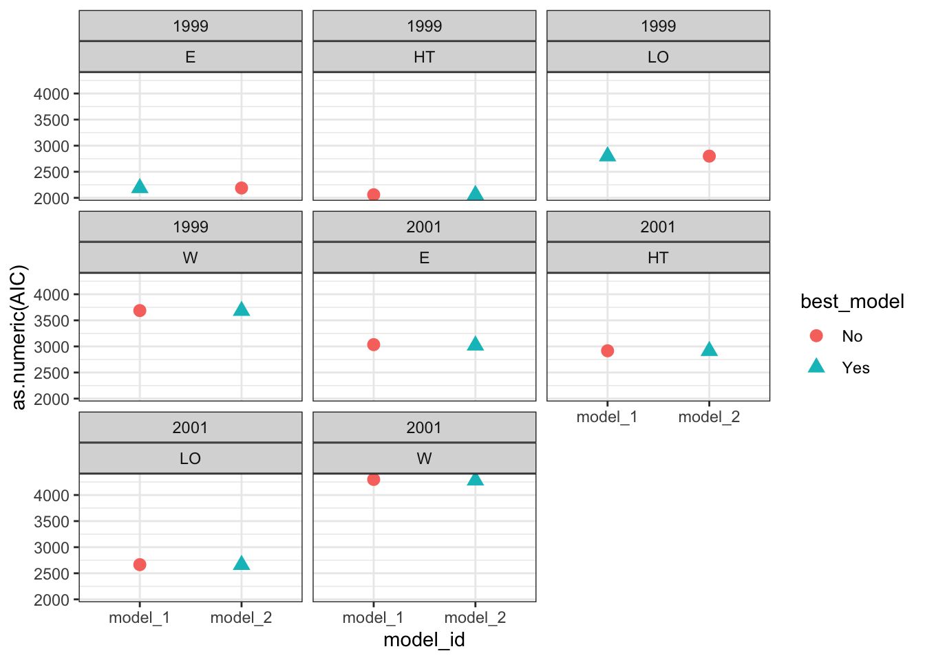
6.5 Model selection

Compare models performance

Show code

# Visual model selection
best_models <- 
  models %>% 
  group_by(year, topo) %>% 
  # Use case_when to identify the best model
  mutate(best_model = 
           case_when(AIC == min(as.numeric(AIC)) ~ "Yes",
                     TRUE ~ "No")) %>% 
  ungroup()

# Plot
best_models %>% 
  ggplot()+
  geom_point(aes(x = model_id, y = as.numeric(AIC), 
                 color = best_model, shape = best_model), 
             size = 3)+
  facet_wrap(year~topo)+
  theme_bw()

Show code

# Final models
selected_models <- best_models %>% dplyr::filter(best_model == "Yes")

6.6 Run ANOVA

Estimate the effects of factor under study

Show code

models_effects <- 
  selected_models %>%
  # Type 3 Sum of Squares (Partial SS, when interactions are present)
  mutate(ANOVA = map(model, ~Anova(., type = 3)) )

# Extract ANOVAS
models_effects$ANOVA[[1]]

Analysis of Deviance Table (Type III tests)

Response: yield
              Chisq Df Pr(>Chisq)    
(Intercept) 5729.95  1  < 2.2e-16 ***
nf           164.03  5  < 2.2e-16 ***
---
Signif. codes:  0 '***' 0.001 '**' 0.01 '*' 0.05 '.' 0.1 ' ' 1

Show code

models_effects$ANOVA[[2]]

Analysis of Deviance Table (Type III tests)

Response: yield
              Chisq Df Pr(>Chisq)    
(Intercept) 6089.64  1  < 2.2e-16 ***
nf           318.03  5  < 2.2e-16 ***
---
Signif. codes:  0 '***' 0.001 '**' 0.01 '*' 0.05 '.' 0.1 ' ' 1

Show code

models_effects$ANOVA[[3]]

Anova Table (Type III tests)

Response: yield
            Sum Sq  Df  F value    Pr(>F)    
(Intercept) 158985   1 7299.604 < 2.2e-16 ***
nf            1975   5   18.136 4.699e-16 ***
rep            691   2   15.858 2.509e-07 ***
Residuals     7841 360                       
---
Signif. codes:  0 '***' 0.001 '**' 0.01 '*' 0.05 '.' 0.1 ' ' 1

Show code

models_effects$ANOVA[[8]]

Analysis of Deviance Table (Type III tests)

Response: yield
                Chisq Df Pr(>Chisq)    
(Intercept) 18282.203  1  < 2.2e-16 ***
nf             72.431  5  3.194e-14 ***
---
Signif. codes:  0 '***' 0.001 '**' 0.01 '*' 0.05 '.' 0.1 ' ' 1

6.7 Means comparison

Show code

# MULTCOMPARISON
# emmeans and cld multcomp
# We need to specify ourselves the most important interaction to perform the comparisons
mult_comp <- 
  models_effects %>% 
  dplyr::filter(topo == "HT") %>% 
  # Comparisons estimates (emmeans)
  mutate(mc_estimates = map(.x=model, ~emmeans(object=.x, ~ nf))) %>% 
  # Assign letters and p-value adjustment (multcomp)
  mutate(mc_letters = 
           map(mc_estimates, 
               ~as.data.frame( 
                 # By specifies a strata or level to assign the letters
                 cld(object=., decreasing = TRUE, details=FALSE,
                     reversed=TRUE, alpha=0.05,  adjust = "tukey", Letters=letters))))

7 Plotting

We can also use mapping to create multiple plots at once. ## data preparation

Show code

# Unnest data
data_plot <- data_corn_00

7.1 plotting function

Show code

plot_yield_vs_nitro <- 
  function(data, x_var, y_var, group_var, facet_var,
           smooth_method = "loess", se = FALSE, title = NULL) {

  ggplot(data, aes_string(x = x_var, y = y_var)) +
    geom_point(aes_string(color = group_var, fill = group_var, shape = group_var),
               size = 2, alpha = 0.85) +
    geom_smooth(aes_string(color = group_var, fill = group_var),
                method = smooth_method, se = se) +
    scale_color_brewer(palette = "Set1") +
    scale_fill_brewer(palette = "Set1") +
    facet_wrap(as.formula(paste("~", facet_var))) +
    theme_bw() +
    labs(
      title = title,
      x = x_var,
      y = y_var,
      color = group_var,
      fill  = group_var,
      shape = group_var
    )
}

We can also pass options for plots as vectors or list

Show code

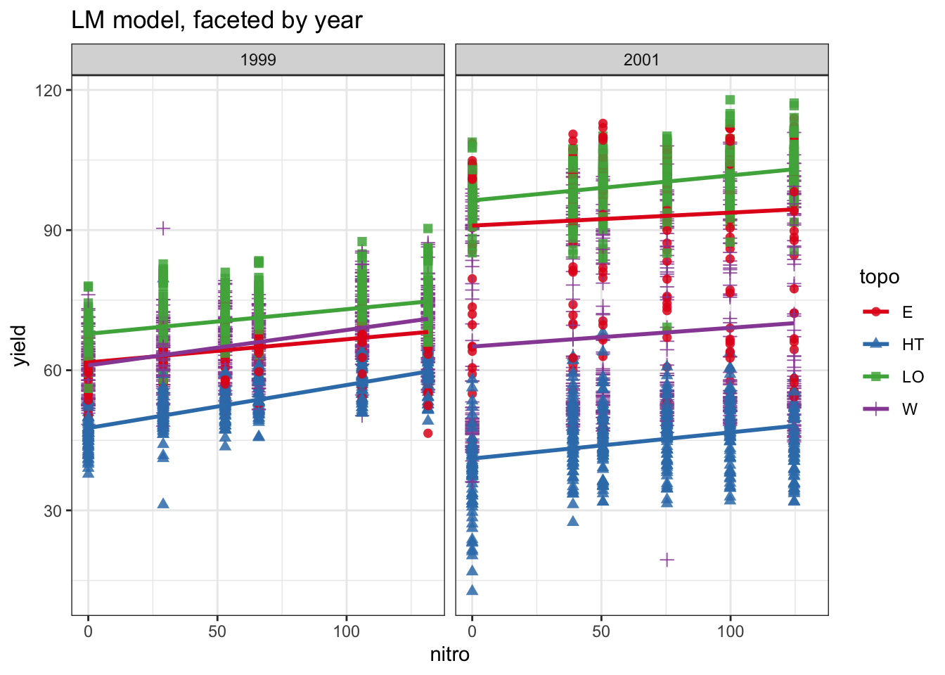
methods <- c("loess", "lm")
ses     <- c(TRUE, FALSE)
titles  <- c("LOESS model, faceted by year",
             "LM model, faceted by year")

7.2 Create plots with `pmap()`

Show code

plots <- pmap(
  list(
    smooth_method = methods,
    se = ses,
    title = titles,
    facet_var = rep("year", length(methods)),
    group_var = rep("topo", length(methods))
  ),
  function(smooth_method, se, title, facet_var, group_var) {
    plot_yield_vs_nitro(
      data = data_plot,
      x_var = "nitro",
      y_var = "yield",
      group_var = group_var,
      facet_var = facet_var,
      smooth_method = smooth_method,
      se = se,
      title = title
    )
  }
)

Warning: `aes_string()` was deprecated in ggplot2 3.0.0.
ℹ Please use tidy evaluation idioms with `aes()`.
ℹ See also `vignette("ggplot2-in-packages")` for more information.

7.3 Display plots

Show code

# use walk to print them all at once
walk(.x=plots, .f=print)

`geom_smooth()` using formula = 'y ~ x'

`geom_smooth()` using formula = 'y ~ x'

8 Final comments

Iteration is a fundamental skill in data science, and purrr provides an expressive, efficient, and tidy approach to iteration. By using map(), map2(), and pmap(), we can iterate over multiple variables seamlessly, avoiding verbose loops while improving readability and maintainability.

8.0.1 Further Resources

Happy coding!

1 Introduction to Iteration

2 Traditional for Loop Example

3 Using purrr::map() for Iteration

4 Comparison of For Loops and Mapping Functions

4.1 Understanding the Difference Between map() and map_dbl()

5 Using the purrr Package for Iteration

5.1 Practical Application

6 Working with the agridat Dataset

6.1 Load the data

6.2 Prepare the data

6.3 Create functions

6.3.1 Rep (block) as fixed

6.3.2 Rep (block) as random

6.4 Fit models with mapping

6.5 Model selection

6.6 Run ANOVA

6.7 Means comparison

7 Plotting

7.1 plotting function

7.2 Create plots with pmap()

7.3 Display plots

8 Final comments

8.0.1 Further Resources

2 Traditional `for` Loop Example

3 Using `purrr::map()` for Iteration

4.1 Understanding the Difference Between `map()` and `map_dbl()`

5 Using the `purrr` Package for Iteration

6 Working with the `agridat` Dataset

7.2 Create plots with `pmap()`