Intro to Bayesian Statistics

Intro

This article provides some basics about Bayesian statistics and a comparison with the conventional frequentist perspective about probabilities and statistical inference.

Important

Neither Frequentist nor Bayesian approaches are universally superior. Each has strengths, limitations, and situations where it is more useful.

1 Why should we care?

In agricultural research, we rarely work with perfect data. We often deal with small sample sizes, noisy field conditions, site-year variation, and previous knowledge coming from earlier trials, expert opinion, or long-term experiments.

Because of that, statistics is not just about computing a p-value. It is about learning from data while being honest about uncertainty.

Bayesian statistics offers one way to do that. It is not magic, and it is not automatically better than conventional methods. But it gives us a useful framework to combine previous knowledge with observed data and express uncertainty in a direct way.

Today, we will compare the Frequentist and Bayesian perspectives, and discuss what each approach can do well (and not so well) for applied agricultural science.

2 Frequentism vs Bayesianism

What are your thoughts?

• Let’s open the floor for discussion!

2.1 Main differences

The key difference lies in where uncertainty is placed.

2.1.1 Frequentist perspective

In Frequentist statistics, parameters are treated as fixed but unknown, and randomness comes from the data-generating process.

It is called frequentist because probability is defined in terms of long-run frequencies under repeated sampling.

🎲 Example: To estimate the probability of rolling a 6, a Frequentist would say: “If we rolled the die many times under the same conditions, the proportion of 6s would approach its true probability.”

So the logic of inference is based on hypothetical repetition of the same experiment.

2.1.2 Bayesian perspective

In Bayesian statistics, unknown quantities are treated as uncertain, and that uncertainty is represented with probability distributions.

This does not mean truth does not exist. It means that, before observing enough data, we describe our uncertainty about the unknown using probability.

For example, if the probability of rolling a 6 is unknown, we may call it \(\theta\) and assign a prior distribution to \(\theta\). After observing data, we update that prior into a posterior distribution.

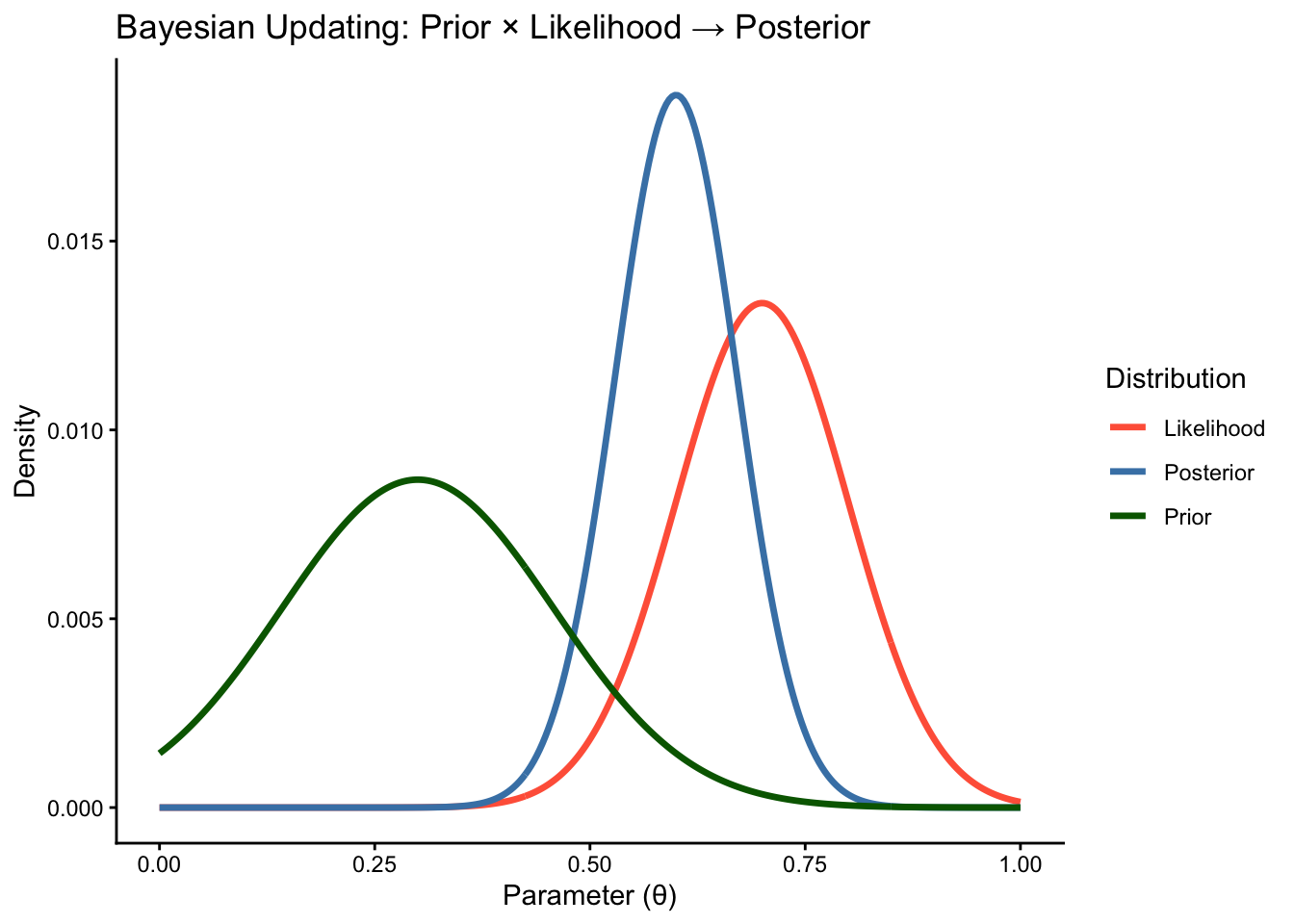
Bayesian inference is built around the idea of updating beliefs with data:

\[ \text{Posterior} = \frac{\text{Likelihood} \times \text{Prior}}{\text{Evidence}} \]

2.1.3 Summary

• Frequentist: parameters are fixed but unknown; data are random under repeated sampling.
• Bayesian: observed data are fixed; uncertainty about parameters is represented by prior and posterior distributions.

Tip

For many simple models, both approaches often lead to similar practical conclusions, especially when the dataset is large and priors are weak.

3 Probability and conditional thinking

One of the most attractive features of Bayesian statistics is that it makes inference explicitly conditional.

A conditional probability such as

\[ P(A \mid B) \]

is read as:

the probability of \(A\), given that \(B\) is known.

This idea is familiar in everyday reasoning. For example:

• \(P(\text{disease} \mid \text{positive test})\)
• \(P(\text{rain tomorrow} \mid \text{current weather conditions})\)

In Bayesian inference, we are interested in quantities such as:

\[ P(\theta \mid y) \]

where:

• \(\theta\) is an unknown parameter
• \(y\) is the observed data

This is read as:

the probability distribution of the parameter, given the observed data.

That is the core of Bayesian inference.

Note

Bayesian conclusions are always conditional on:

1. the observed data,
2. the statistical model,
3. and the prior assumptions.

So Bayesian inference is not assumption-free. It is explicit about the assumptions used to update uncertainty.

4 Bayes’ theorem

Bayes’ theorem gives the mathematical rule for updating our beliefs:

\[ P(\theta \mid y) = \frac{P(y \mid \theta) \cdot P(\theta)}{P(y)} \]

or, in words,

\[ \text{Posterior} = \frac{\text{Likelihood} \times \text{Prior}}{\text{Evidence}} \]

where:

• Prior: what we assumed or believed before seeing the data
• Likelihood: how compatible different parameter values are with the observed data
• Evidence: a scaling constant that makes the posterior a proper probability distribution
• Posterior: our updated belief after observing the data

4.1 Video: Bayes’ Rule

5 The priors

Priors formalize previous information or assumptions as probability distributions.

They can be based on:

1. the nature of the variable (discrete or continuous),
2. previous experiments,
3. expert knowledge,
4. or deliberately weak assumptions when prior information is limited.

Tip

In practice, analysts often use weakly informative priors when they want the data to dominate the analysis while still ruling out unreasonable parameter values.

A prior is not necessarily subjective guesswork. In many applied problems, it can represent previous field trials, historical datasets, or realistic agronomic constraints.

At the same time, priors should not be treated carelessly. With limited data, they can influence results strongly.

6 A simple agronomic example

Suppose we want to estimate the economically optimum nitrogen rate (EONR) for corn.

A Frequentist approach might fit a response curve and produce a point estimate and confidence interval for EONR.

A Bayesian approach could do the same, but it can also:

• incorporate previous site-years as prior information,
• express uncertainty in EONR directly through a posterior distribution,
• and naturally extend to hierarchical models across years, sites, hybrids, or landscape positions.

So instead of only reporting a single estimate, we could describe our updated uncertainty about the optimum nitrogen rate as:

\[ P(\text{EONR} \mid \text{data}) \]

That is, our inference about EONR is conditional on both the observed data and the assumptions used in the model.

7 Visualization of Bayesian updating

The following figure is a conceptual sketch of Bayesian updating. It is meant to illustrate the idea of combining prior information with observed data through the likelihood to obtain a posterior distribution.

x <- seq(0, 1, length.out = 300)
prior <- exp(-((x - 0.3)^2) / 0.05)
likelihood <- exp(-((x - 0.7)^2) / 0.02)
posterior <- exp(-((x - 0.6)^2) / 0.01)

# Normalize
prior <- prior / sum(prior)
likelihood <- likelihood / sum(likelihood)
posterior <- posterior / sum(posterior)

df <- data.frame(x = x, Prior = prior, Likelihood = likelihood, Posterior = posterior)

df_long <- df %>% 
  pivot_longer(cols = -x, names_to = "Distribution", values_to = "Density")

ggplot(df_long, aes(x = x, y = Density, color = Distribution)) +
  geom_line(linewidth = 1.2) +
  labs(title = "Bayesian Updating: Prior × Likelihood → Posterior",
       x = "Parameter (θ)", y = "Density") +
  theme_classic() +
  scale_color_manual(values = c("tomato", "steelblue", "darkgreen"))

Fig 1. Conceptual sketch of Bayesian updating: Prior × Likelihood → Posterior

8 Credible intervals vs confidence intervals

A common source of confusion in statistics is the interpretation of intervals.

• Confidence interval (Frequentist): If we repeated the experiment many times under the same conditions, 95% of the intervals produced by that method would contain the true parameter value.

  The parameter is treated as fixed. The interval procedure has a long-run success rate of 95%.

• Credible interval (Bayesian): Given the observed data, the model, and the prior assumptions, there is a 95% probability that the parameter lies within the interval.

  This interpretation is often more intuitive, but it is conditional on the model and prior assumptions.

9 Bayes factor and model comparison

When comparing two competing models, Bayesians may use the Bayes factor, which measures how much more strongly the observed data support one model over another:

\[ BF_{10} = \frac{P(\text{data} \mid M_1)}{P(\text{data} \mid M_0)} \]

A Bayes factor greater than 1 favors model \(M_1\), whereas a value less than 1 favors model \(M_0\).

A useful way to understand this is through odds:

\[ \text{Posterior odds} = \text{Prior odds} \times \text{Bayes factor} \]

or equivalently,

\[ \frac{P(M_1 \mid \text{data})}{P(M_0 \mid \text{data})} = \frac{P(M_1)}{P(M_0)} \times \frac{P(\text{data} \mid M_1)}{P(\text{data} \mid M_0)} \]

So:

• prior odds represent what we believed before seeing the data,
• Bayes factor represents what the data contributed,
• posterior odds represent our updated support for one model relative to another.

Note

For an introductory course, Bayes factors are helpful mainly as a model-comparison concept. They are not required to understand the basic prior-likelihood-posterior workflow.

10 The good, the bad, and the ugly

10.1 Frequentist approaches

10.1.1 The good

• Widely taught and widely used
• Many standard tools work very well for common agronomic experiments
• Straightforward workflows for familiar analyses such as ANOVA, regression, and mixed models

10.1.2 The bad

• P-values are often over-interpreted
• Confidence intervals are commonly explained incorrectly
• Results are sometimes reduced to a simple significant/non-significant decision

10.1.3 The ugly

• Mechanical threshold thinking can replace scientific judgment
• Statistical significance can be confused with agronomic relevance
• Selective reporting and p-hacking can distort conclusions

10.2 Bayesian approaches

10.2.1 The good

• Probability statements about parameters are often more intuitive
• Prior information can be incorporated formally
• Very flexible for hierarchical models, small datasets, and complex uncertainty structures

10.2.2 The bad

• Requires more modeling decisions
• Priors can affect results, especially when data are limited
• Computation can be slower and model checking can be more demanding

10.2.3 The ugly

• Poorly chosen priors plus weak data can be misleading
• Complex Bayesian models can create a false sense of rigor
• It is easy to trust software output without checking convergence, model fit, and sensitivity to priors

11 Final thoughts

Bayesian statistics is not a replacement for good scientific thinking, and it is not automatically superior to frequentist methods.

Its main value is that it gives us a coherent way to combine prior information, observed data, and uncertainty into a single inferential framework.

In many simple problems, Frequentist and Bayesian approaches may lead to similar answers. The real advantage of Bayesian methods often becomes clearer when:

• data are limited,
• multilevel structure matters,
• previous knowledge is relevant,
• or decision-making under uncertainty is central.

For applied agricultural science, the best method is usually the one that matches the research question, the structure of the data, and the kind of uncertainty we need to communicate.

12 Useful resources

12.1 Introductory theory

• Bayesian Models: A Statistical Primer for Ecologists – Hobbs & Hooten
• Bringing Bayesian Models to Life – Hooten & Hefley
• Statistical Rethinking – McElreath (PDF)

12.2 Bayesian workflow and philosophy

• Bayesian workflow – Gelman et al.
• Scientific Reasoning: The Bayesian Approach – Howson & Urbach

12.3 Advanced theory

• Bayesian Data Analysis (3rd Edition)

12.4 Agronomy applications

• Makowski et al., 2020 (EJA) Analyzing uncertainty in critical nitrogen dilution curves
  
• Correndo et al., 2021 (Ag. For. Meteorol.) Unraveling uncertainty drivers of the maize yield response to nitrogen: A Bayesian and machine learning approach.
  
• Lacasa et al., 2020 (Sci. Rep.) Bayesian approach for maize yield response to plant density from both agronomic and economic viewpoints in North America
  
• Palmero et al., 2024 (Plant Methods) A Bayesian approach for estimating the uncertainty on the contribution of nitrogen fixation and calculation of nutrient balances in grain legumes
  
• Giordano et al. 2025 (Plant Methods) A Bayesian framework to model variance of grain yield response to plant density
  

12.5 Miscellaneous

• Statistical Modeling Blog – Gelman et al.
• Learning Bayesian Statistics Podcast