library(pacman)
p_load("readxl") # To open/save excel files
p_load('dplyr', "tidyr","purrr", "forcats", "stringr") # Data wrangling
p_load("nlme") # Mixed models libraries
p_load("broom", "broom.mixed") # Managing models results
p_load("performance") # Check assumptions and performance
p_load("emmeans","multcomp","multcompView",
"car") # Aov and mult comp
p_load("ggplot2") # Figures
p_load(tidybayes) # ggplot themeModels IV: Mixed Models II
linear models
R
statistics
agriculture
Summary
This tutorial provides a tidy workflow to analyze another case of common mixed model in agriculture: Repeated-measures.
1 What are repeated measures models?
Repeated measures models are a type of statistical model used when the same experimental unit is measured multiple times under different conditions or over time. These models account for the fact that repeated observations from the same unit (e.g., plant, plot, soil location) are not independent but correlated.
In agriculture, repeated measures designs are common in various scenarios, including:
•   Time-based measurements: Tracking crop growth, soil nutrients, or yield over multiple time points. Or also treatments applied to the same unit over time such as fertilization trials where the same plots receive different treatments over multiple years.
•   Spatially repeated measurements: Soil properties at different depths, plant characteristics at multiple canopy levels, or yield components across field zones.
1.1 Mixed Models for Repeated Measures
Linear mixed models (LMMs) are typically used for analyzing repeated measures because they allow us to include: 1. Fixed effects – Factors of interest, such as treatments, depths, or environmental conditions. 2. Random effects – Sources of variability, such as plot-to-plot differences or repeated observations on the same soil core.
2 Case Study
Today, we are going to reproduce the analysis I’ve performed myself for one of my publications few years ago (Correndo et al. 2021). Particularly, we are going to reproduce Figure 2

For this paper, we have data from 4 different locations. We tested the levels of soil potassium fertility, hereinafter as soil test K (STK), in long-term experiments (2000-2009) where the treatments of interest were: (i) Control (unfertilized), (ii) NPS (fertilized with NPS), and (iii) Pristine conditions (No Ag-history).
At each plot/sample, the STK was measured at five-consecutive soil depths (0-20, 20-40, 40-60, 60-80, and 80-100 cm). Thus, they we took “repeated measurements” over the space.
We were NOT interested in comparing locations since they had very different previous history, and crop rotation, so confounding effects may have obscured the inference. Therefore, site was not a factor under consideration, and all the analysis were fitted independently by site.
2.1 Required packages for today
2.2 Miscellaneous
# Make sure Type-III-like tests behave as expected when you use them
# (only relevant if you insist on car::Anova)
options(contrasts = c("contr.sum", "contr.poly"))

# Base ggplot theme (your earlier set_theme() line is not a ggplot2 function)
ggplot2::theme_set(theme_tidybayes())
2.3 Data
# Read data
# File online? Try this...
url_rm <- "https://raw.githubusercontent.com/adriancorrendo/tidymixedmodelsweb/refs/heads/master/data/02_repeated_measures_data.csv"

# Read file
rm_data_00 <- read.csv(url_rm)

rm_data_01 <-
  rm_data_00 %>%
  # We need to create PLOT column to identify subject (Exp. Unit for Rep. Measures)
  ## Option 1, use "unite"
  unite(data = ., col = PLOT, BLOCK,TREAT, sep = "_", remove=FALSE) %>%
  # OR
  ## Option 2, use cur_group_id
  # Identify Subplot
  ungroup() %>%
  group_by(BLOCK, TREAT) %>% # Don't need to add SITE here
  # Create unique plot ID # Needed for Repeated Measures
  mutate(plot = cur_group_id(), .after = PLOT) %>%
  ungroup() %>%
  ## Transform to factor if needed
  mutate(depth = as.integer(DEPTH), # Needed for CorAR1
         DEPTH = as.factor(DEPTH),
         plot = factor(plot),
         BLOCK = factor(BLOCK),
         SITE = factor(SITE),
                       #levels = c("site_1", "site_2", "site_3", "site_4"),
                       #labels = c("Balducchi", "San Alfredo", "La Blanca", "La Hansa")
         TREAT = factor(TREAT)
         )
2.4 Exploratory analysis
Now, let’s use several functions to explore the data.
2.4.1 misc
# Define your own colors
my_colors <- c("#ffaa00", "#7E5AA0", "#5c9c8c")
2.4.2 glimpse()
First, the glimpse() function from dplyr
# Glimpse from dplyr
dplyr::glimpse(rm_data_01)
Rows: 180
Columns: 8
$ SITE <fct> site_1, site_1, site_1, site_1, site_1, site_1, site_1, site_1, …
$ PLOT <chr> "I_Control", "I_Control", "I_Control", "I_Control", "I_Control",…
$ plot <fct> 1, 1, 1, 1, 1, 4, 4, 4, 4, 4, 7, 7, 7, 7, 7, 2, 2, 2, 2, 2, 5, 5…
$ TREAT <fct> Control, Control, Control, Control, Control, Control, Control, C…
$ BLOCK <fct> I, I, I, I, I, II, II, II, II, II, III, III, III, III, III, I, I…
$ DEPTH <fct> 10, 30, 50, 70, 90, 10, 30, 50, 70, 90, 10, 30, 50, 70, 90, 10, …
$ STK <int> 105, 83, 103, 110, 127, 119, 98, 106, 107, 109, 132, 100, 96, 10…
$ depth <int> 10, 30, 50, 70, 90, 10, 30, 50, 70, 90, 10, 30, 50, 70, 90, 10, …2.4.3 skim()
Then, the skim() function from skmir
# Skim from skimr
skimr::skim(rm_data_01)| Name | rm_data_01 |
| Number of rows | 180 |
| Number of columns | 8 |
| _______________________ | |
| Column type frequency: | |
| character | 1 |
| factor | 5 |
| numeric | 2 |
| ________________________ | |
| Group variables | None |
Variable type: character
| skim_variable | n_missing | complete_rate | min | max | empty | n_unique | whitespace |
|---|---|---|---|---|---|---|---|
| PLOT | 0 | 1 | 5 | 12 | 0 | 9 | 0 |
Variable type: factor
| skim_variable | n_missing | complete_rate | ordered | n_unique | top_counts |
|---|---|---|---|---|---|
| SITE | 0 | 1 | FALSE | 4 | sit: 45, sit: 45, sit: 45, sit: 45 |
| plot | 0 | 1 | FALSE | 9 | 1: 20, 2: 20, 3: 20, 4: 20 |
| TREAT | 0 | 1 | FALSE | 3 | Con: 60, NPS: 60, Pri: 60 |
| BLOCK | 0 | 1 | FALSE | 3 | I: 60, II: 60, III: 60 |
| DEPTH | 0 | 1 | FALSE | 5 | 10: 36, 30: 36, 50: 36, 70: 36 |
Variable type: numeric
| skim_variable | n_missing | complete_rate | mean | sd | p0 | p25 | p50 | p75 | p100 | hist |
|---|---|---|---|---|---|---|---|---|---|---|
| STK | 0 | 1 | 181.84 | 63.09 | 74 | 138.75 | 174 | 221.25 | 406 | ▅▇▅▂▁ |
| depth | 0 | 1 | 50.00 | 28.36 | 10 | 30.00 | 50 | 70.00 | 90 | ▇▇▇▇▇ |
2.4.4 ggplot()
And let’s use ggplot2 for a better look
# Boxplot
rm_data_01 %>%
  dplyr::select(-depth) %>%
  # Plot
ggplot() +
  # Boxplots
  geom_boxplot(aes(x = reorder(DEPTH, desc(DEPTH)), y = STK, fill = TREAT))+
  scale_fill_manual(name="Scenario", values = my_colors,  guide='legend')+
  # Axis labels
  labs(x = "Soil depth (cm)", y = "STK (g/m2)")+
  # Plot by site
  facet_wrap(~SITE)+
  # Flip axes
  coord_flip()+
  # Set scale type
  scale_x_discrete()+
  # Change theme
  tidybayes::theme_tidybayes()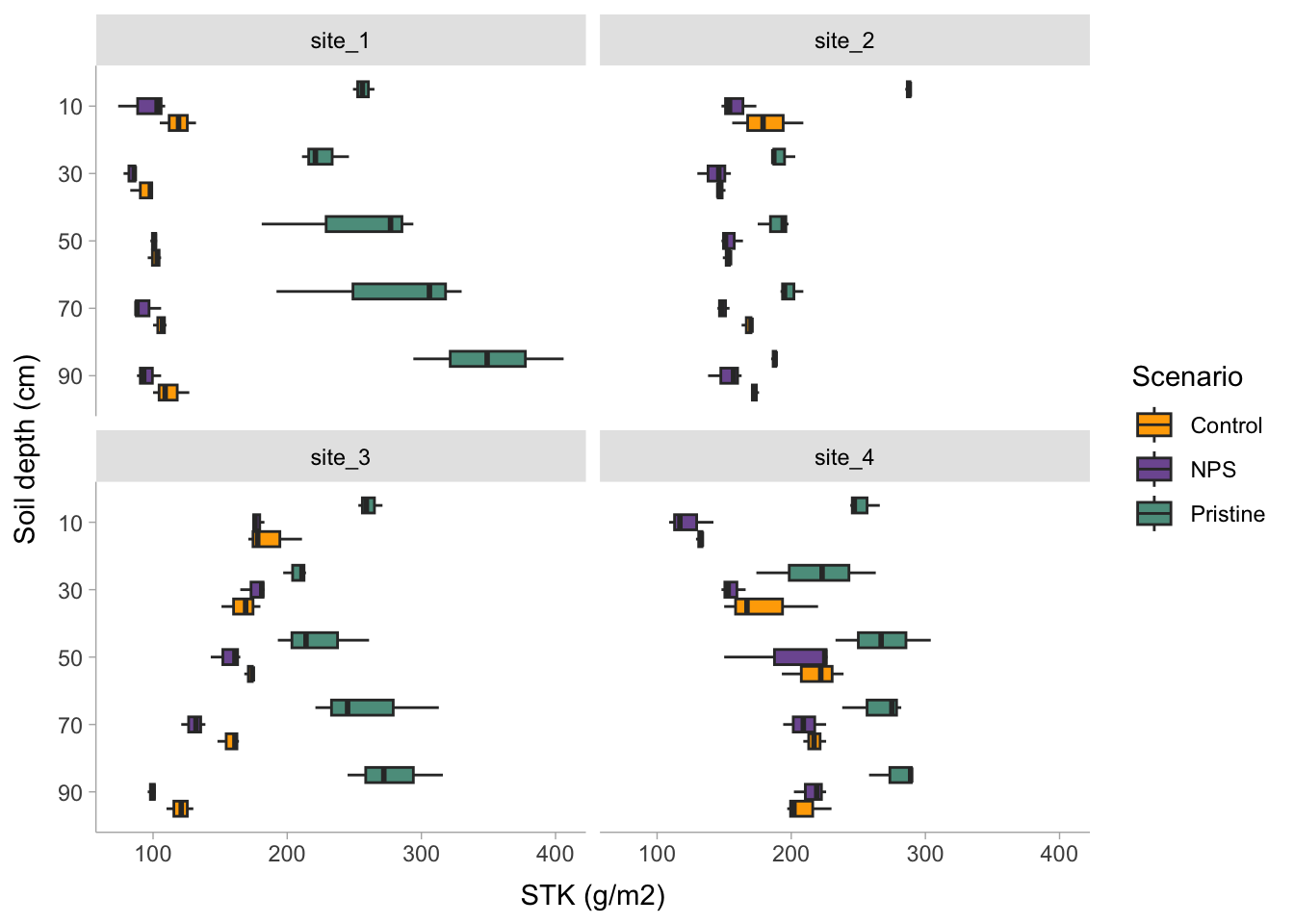
2.4.5 Additional data manipulation?
rm_data_02 <-rm_data_01 %>%
  # Create a grouping variable (WHY?) # Needed for HetVar
  mutate(GROUP = case_when(TREAT == "Pristine" ~ "Pristine",
                           TRUE ~ "Agriculture"))
2.5 Candidate Models
I’m sorry for this, but the most important step is ALWAYS to write down the model.
2.5.1 Formulae
2.5.1.1 m0. Block Fixed
In a traditional approach blocks are defined as fixed, affecting the mean of the expected value. Yet there is no consensus about treating blocks as fixed or as random. For more information, read Dixon (2016).
Let’s define the model. For simplification (and avoid writing interaction terms), here we are going to consider that \(\tau_i\) is the “treatment”.
\[ y_{ij} = \mu + \tau_i + \beta_j + \epsilon_{ij} \]
\[ \epsilon_{ij} \sim N(0, \sigma^2_{e} )\] where \(\mu\) represents the overall mean (if intercept is used), \(\tau_i\) is the effect of treatment-j over \(\mu\), \(\beta_j\) is the effect of block-j over \(\mu\), and \(\epsilon_{ij}\) is the random effect of each experimental unit.
# SIMPLEST MODEL
fit_block_fixed <- function(x){
  lm(# Response variable
     STK ~
       # Fixed
       TREAT + DEPTH + TREAT:DEPTH + BLOCK,
     # Data
     data = x)
  }
2.5.1.2 m1. Block Random
An alternative approach is considering a MIXED MODEL, where blocks are considered “random”. Basically, we add a term to the model that it is expected to show a “null” overall effect over the mean of the variable of interest but introduces “noise”. By convention, a random effect is expected to have an expected value equal to zero but a positive variance as follows: \[ y_{ij} = \mu + \tau_i + \beta_j + \epsilon_{ij} \] \[ \beta_j \sim N(0, \sigma^2_{b} )\] \[ \epsilon_{ij} \sim N(0, \sigma^2_{e} )\] Similar than before, \(\mu\) represents the overall mean (if intercept is used), \(\tau_i\) is the effect of treatment-j over \(\mu\), \(\beta_j\) is the “random” effect of block-j over \(\mu\), and \(\epsilon_{ij}\) is the random effect of each experimental unit.
So what’s the difference? Simply specifying this component: \[ \beta_j \sim N(0, \sigma^2_b) \], which serves to model the variance.
How do we write that?
# RANDOM BLOCK
fit_block_random <- function(x){
  nlme::lme(
    # Fixed
    STK ~ TREAT + DEPTH + TREAT:DEPTH,
    # Random
    random = ~1|BLOCK,
    # Data
    data = x)
}2.5.3 Fit
Run the candidate models
STK_models <-
  rm_data_02 %>%
  # Let's group data to run multiple locations|datasets at once
  group_by(SITE) %>%
  # Store the data per location using nested arrangement
  nest() %>%
  # BLOCK as FIXED
  mutate(model_0 = map(data, fit_block_fixed)) %>%
  # BLOCK as RANDOM
  mutate(model_1 = map(data, fit_block_random)) %>%
  # COMPOUND SYMMETRY
  mutate(model_2 = map(data, fit_corsymm)) %>%
  # AUTO-REGRESSIVE ORDER 1
  mutate(model_3 = map(data, fit_ar1)) %>%
  # COMPOUND SYMMETRY + HETEROSKEDASTIC
  mutate(model_4 = map(data,  fit_corsymm_hetvar) ) %>%

  # Data wrangling
  pivot_longer(cols = c(model_0:model_4), # show alternative 'contains' model
               names_to = "model_id",
               values_to = "model") %>%
  # Map over model column
  mutate(results = map(model, broom.mixed::augment )) %>%
  # Performance
  mutate(performance = map(model, broom.mixed::glance )) %>%
  # Extract AIC
  mutate(AIC = map(performance, ~.x$AIC)) %>%
  # Extract coefficients
  mutate(coef = map(model, ~coef(.x))) %>%
  # Visual-check plots
  mutate(checks = map(model, ~performance::check_model(.))) %>%
  ungroup()
2.5.4 Check assumptions
Checking assumptions is always important. To learn more about data exploration, tools to detect outliers, heterogeneity of variance, collinearity, dependence of observations, problems with interactions, among others, I highly recommend reading (Zuur, Ieno, and Elphick 2010).
# Extracting by site
site_1_models <- STK_models %>% dplyr::filter(SITE == "site_1")
site_2_models <- STK_models %>% dplyr::filter(SITE == "site_3")
site_3_models <- STK_models %>% dplyr::filter(SITE == "site_4")
site_4_models <- STK_models %>% dplyr::filter(SITE == "site_2")(site_1_models %>% dplyr::filter(model_id == "model_0"))$checks[[1]]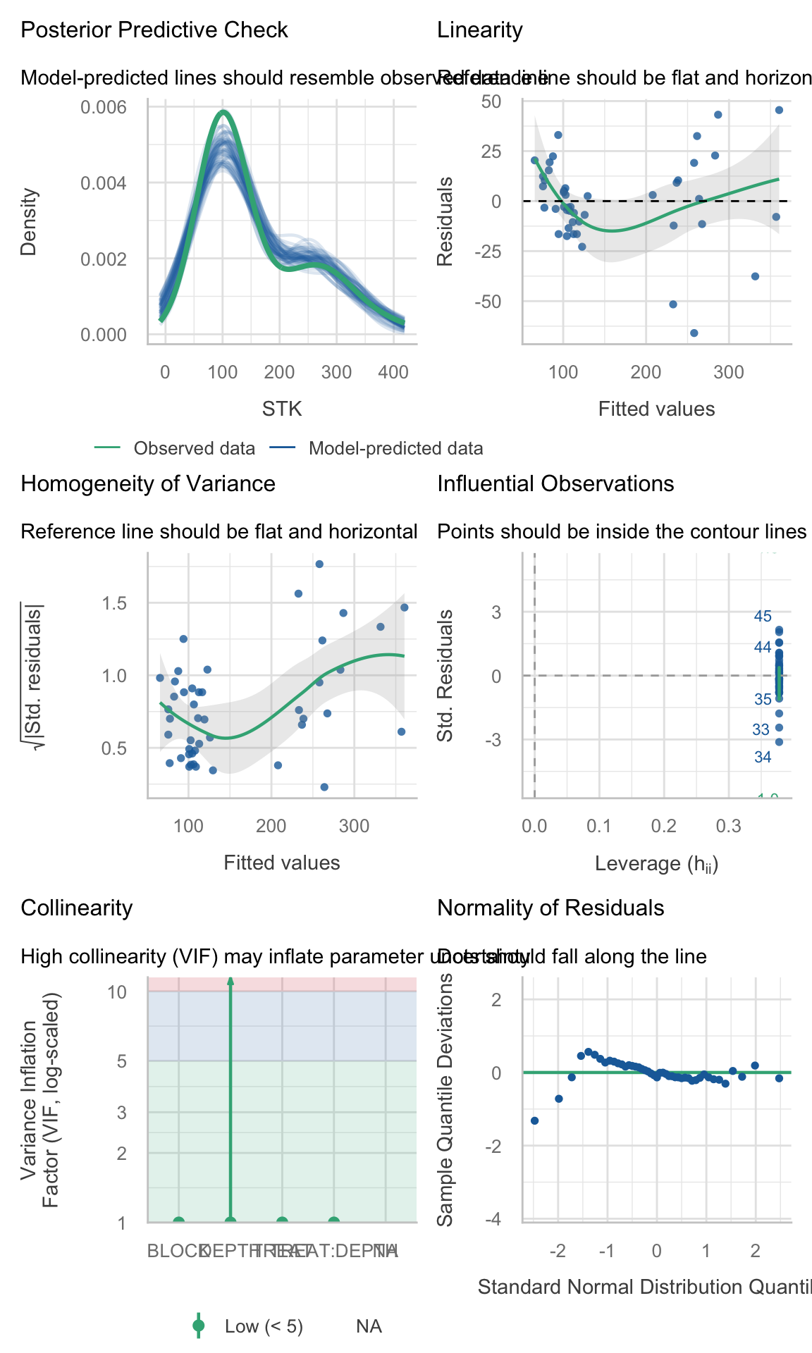
(site_2_models %>% dplyr::filter(model_id == "model_0"))$checks[[1]]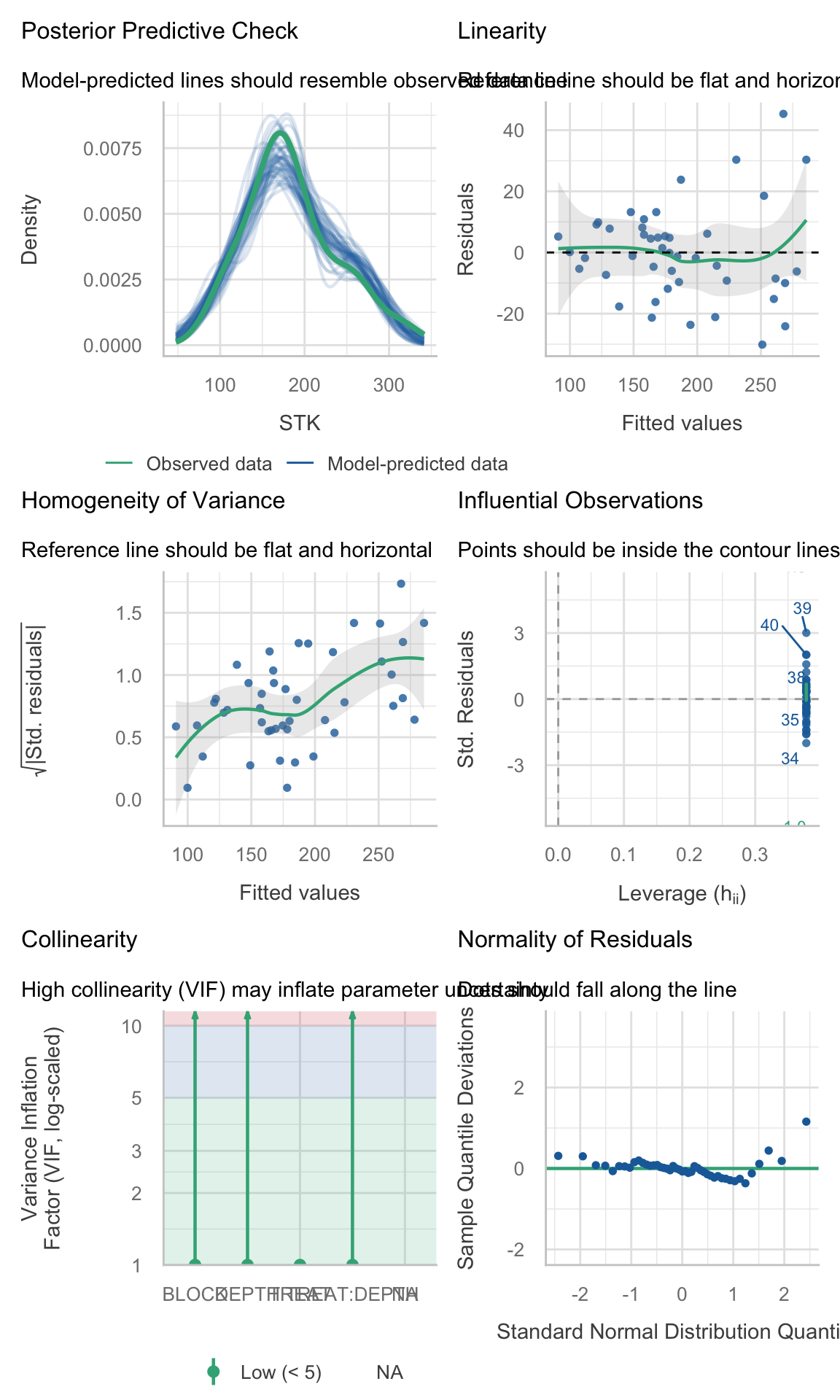
(site_3_models %>% dplyr::filter(model_id == "model_0"))$checks[[1]]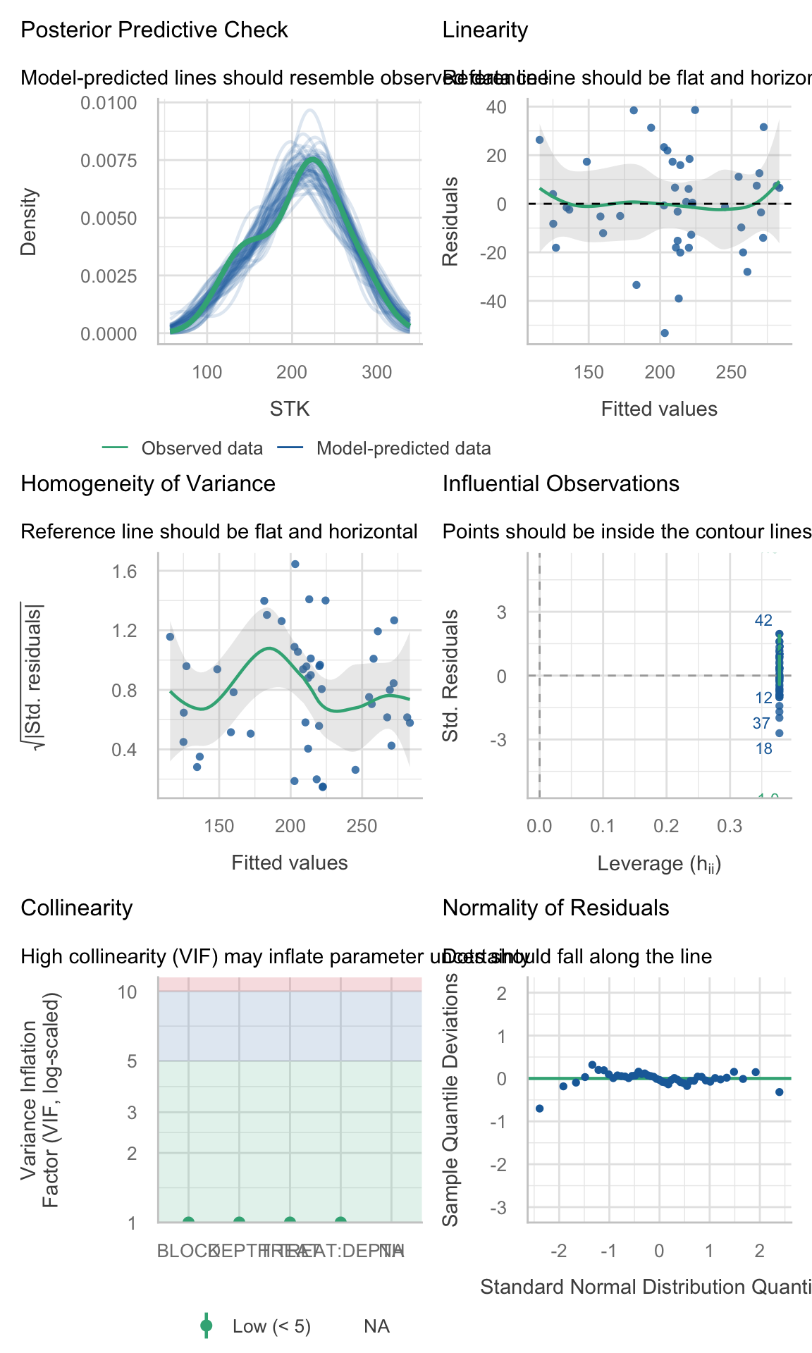
(site_4_models %>% dplyr::filter(model_id == "model_0"))$checks[[1]]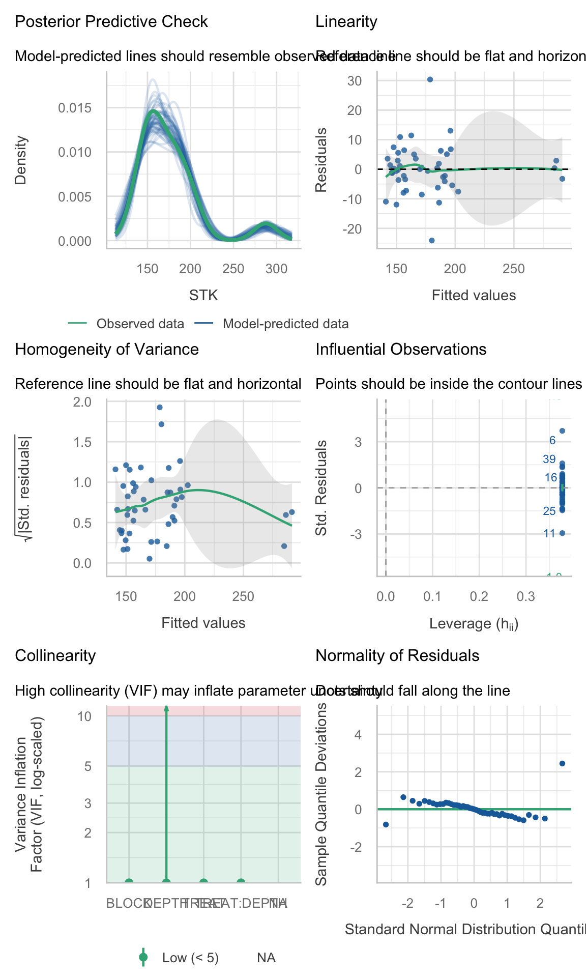
2.5.5 Model Selection
Compare models performance
# Visual model selection
best_STK_models <-
  STK_models %>%
  group_by(SITE) %>%
  # Use case_when to identify the best model
  mutate(best_model =
           case_when(AIC == min(as.numeric(AIC)) ~ "Yes",
                     TRUE ~ "No")) %>%
  ungroup()

# Plot
best_STK_models %>%
  ggplot()+
  geom_point(aes(x = model_id, y = as.numeric(AIC),
                 color = best_model, shape = best_model),
             size = 3)+
  facet_wrap(~SITE)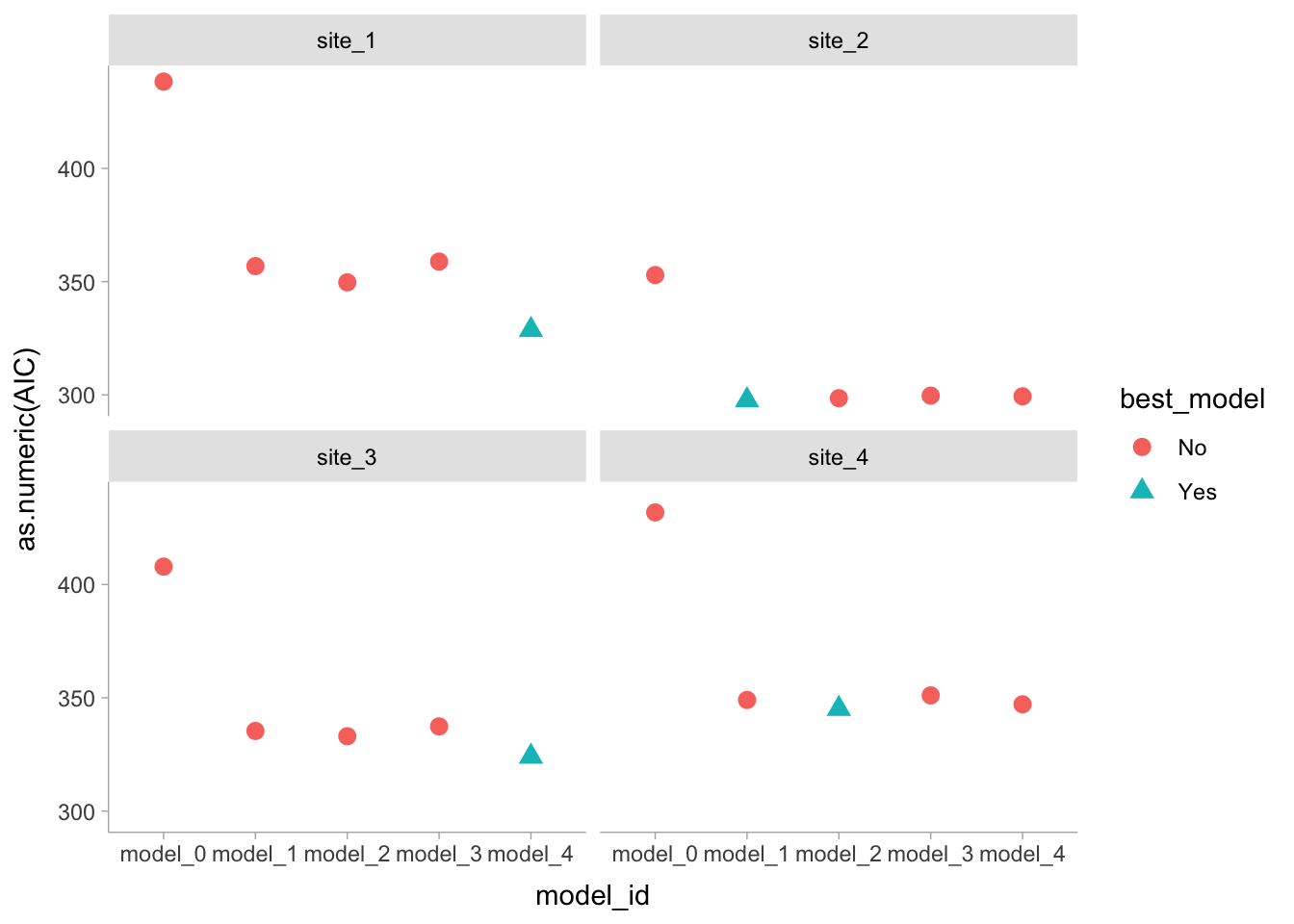
# Final models
selected_models <- best_STK_models %>% dplyr::filter(best_model == "Yes")
2.5.6 Analysis of Variance
It is always recommended to perform an ANOVA to test the significance of the effects. In this case, we are going to use Type III Sum of Squares (Partial SS) since we have interactions in the model.
models_effects <-
  selected_models %>%
  # Type 3 Sum of Squares (Partial SS, when interactions are present)
  mutate(ANOVA = map(model, ~Anova(., type = 3)) )

# Extract ANOVAS
# Site 1
models_effects$ANOVA[[1]]
Analysis of Deviance Table (Type III tests)
Response: STK
Chisq Df Pr(>Chisq)
(Intercept) 660.836 1 < 2.2e-16 ***
TREAT 99.966 2 < 2.2e-16 ***
DEPTH 25.204 4 4.578e-05 ***
TREAT:DEPTH 21.827 8 0.005247 **
---
Signif. codes: 0 '***' 0.001 '**' 0.01 '*' 0.05 '.' 0.1 ' ' 1# Site 2
models_effects$ANOVA[[2]]Analysis of Deviance Table (Type III tests)
Response: STK
Chisq Df Pr(>Chisq)
(Intercept) 2537.803 1 < 2.2e-16 ***
TREAT 89.257 2 < 2.2e-16 ***
DEPTH 26.932 4 2.052e-05 ***
TREAT:DEPTH 52.957 8 1.099e-08 ***
---
Signif. codes: 0 '***' 0.001 '**' 0.01 '*' 0.05 '.' 0.1 ' ' 1# Site 3
models_effects$ANOVA[[3]]Analysis of Deviance Table (Type III tests)
Response: STK
Chisq Df Pr(>Chisq)
(Intercept) 1271.964 1 < 2.2e-16 ***
TREAT 32.783 2 7.608e-08 ***
DEPTH 87.020 4 < 2.2e-16 ***
TREAT:DEPTH 21.773 8 0.005355 **
---
Signif. codes: 0 '***' 0.001 '**' 0.01 '*' 0.05 '.' 0.1 ' ' 1# Site 4
models_effects$ANOVA[[4]]Analysis of Deviance Table (Type III tests)
Response: STK
Chisq Df Pr(>Chisq)
(Intercept) 7704.13 1 < 2.2e-16 ***
TREAT 271.66 2 < 2.2e-16 ***
DEPTH 123.51 4 < 2.2e-16 ***
TREAT:DEPTH 107.84 8 < 2.2e-16 ***
---
Signif. codes: 0 '***' 0.001 '**' 0.01 '*' 0.05 '.' 0.1 ' ' 1However, car::Anova() can’t handle well the models with correlated errors, so we will use the ANOVA tables from the fitted models instead (or emmeans joint tests, see below).
Why we avoid
car::Anova(type = 3) here (and what to do instead)
When we fit repeated-measures models with nlme::lme() (correlated errors via corCompSymm() or corAR1(), and possibly heterogeneous variances via weights = varIdent()), the model is no longer a simple “independent errors” setting. In this situation:
car::Anova(type = 3)can still return a table, but it is a Wald-type test whose degrees-of-freedom handling and interpretation are often confusing in correlated-error models.- With interactions present (e.g.,
TREAT:DEPTH), Type III tables are also easy to misread: the main-effect rows do not answer the main agronomic questions (for example, differences among treatments at each depth), because the interaction implies that treatment effects vary by depth.
Workaround used in this lesson:
Use REML + AIC to choose the covariance/variance structure (fixed effects held constant across candidate models).
Refit the selected model with ML for fixed-effect inference.
2.5.6.1 Refit with ML
selected_models_ml <- selected_models %>%
mutate(model_ML = purrr::map(.x= model , ~update(.x, method = "ML", data = nlme::getData(.x))))- Use
emmeans::joint_tests()for joint tests of model terms, andemmeans()contrasts for the comparisons we actually care about (simple effects and letter displays).
emmeans::joint_tests() is a convenient function that performs joint (Wald) tests for each term in the model, including interactions. It provides a more interpretable output compared to car::Anova(type = 3) when dealing with mixed models with correlated errors.
models_effects_ml <- selected_models_ml %>%
  mutate(
    # Joint (Wald) tests for each term in the model
    joint_tests = map(model_ML, ~emmeans::joint_tests(.x)) )

models_effects_ml$joint_tests[[1]]
model term df1 df2 F.ratio p.value
TREAT 2 28 49.983 <0.0001
DEPTH 4 28 6.301 0.0010
TREAT:DEPTH 8 28 2.728 0.0233models_effects_ml$joint_tests[[2]] model term df1 df2 F.ratio p.value
TREAT 2 28 44.629 <0.0001
DEPTH 4 28 6.733 0.0006
TREAT:DEPTH 8 28 6.620 <0.0001models_effects_ml$joint_tests[[3]] model term df1 df2 F.ratio p.value
TREAT 2 28 16.392 <0.0001
DEPTH 4 28 21.755 <0.0001
TREAT:DEPTH 8 28 2.722 0.0236models_effects_ml$joint_tests[[4]] model term df1 df2 F.ratio p.value
TREAT 2 28 135.828 <0.0001
DEPTH 4 28 30.878 <0.0001
TREAT:DEPTH 8 28 13.480 <0.0001Option B: nlme::anova(type = "marginal")
This is also equivalent. It’s the closest built-in analogue to “partial” tests. Keep it in case the joint tests don’t work for some reason, but emmeans::joint_tests() is perhaps more straightforward and easier to interpret in this context.
models_effects_anova <- selected_models_ml %>%
  mutate(
    anova_marginal = map(model_ML, ~anova(.x, type = "marginal"))
  )

models_effects_anova$anova_marginal[[1]]
numDF denDF F-value p-value
(Intercept) 1 28 660.8356 <.0001
TREAT 2 28 49.9833 <.0001
DEPTH 4 28 6.3010 0.0010
TREAT:DEPTH 8 28 2.7283 0.0233models_effects_anova$anova_marginal[[2]] numDF denDF F-value p-value
(Intercept) 1 28 2537.8035 <.0001
TREAT 2 28 44.6287 <.0001
DEPTH 4 28 6.7330 6e-04
TREAT:DEPTH 8 28 6.6196 1e-04models_effects_anova$anova_marginal[[3]] numDF denDF F-value p-value
(Intercept) 1 28 1271.9683 <.0001
TREAT 2 28 16.3915 <.0001
DEPTH 4 28 21.7550 <.0001
TREAT:DEPTH 8 28 2.7216 0.0236models_effects_anova$anova_marginal[[4]] numDF denDF F-value p-value
(Intercept) 1 28 7704.133 <.0001
TREAT 2 28 135.828 <.0001
DEPTH 4 28 30.878 <.0001
TREAT:DEPTH 8 28 13.480 <.0001- Then we run our multiple comparisons with
emmeans::emmeans(), which are consistent with the fitted model and the questions we want to answer. This keeps inference consistent with the fittednlmemodel and aligns results with the questions we want to answer.
2.5.7 Means comparison
# Means and multiple comparisons are computed directly from the selected nlme model
# (REML is fine here; ML refits are only needed for likelihood-based comparisons of fixed effects).

mult_comp <-
  models_effects %>%
  mutate(
    # EMM grid
    mc_emm = map(model, ~emmeans(., ~ TREAT * DEPTH)),
    # Summary table of means with reasonable (pointwise) CIs
    mc_means = map(mc_emm,~as.data.frame(summary(.x, infer = c(TRUE, TRUE))) ),
    # Compact letter display within each depth (multiple-comparison adjusted)
    mc_letters = map(mc_emm,
                     ~as.data.frame(
                       cld(object = .x,
                           by = "DEPTH",
                           decreasing = TRUE,
                           details = FALSE,
                           reversed = TRUE,
                           alpha = 0.05,
                           adjust = "sidak",
                           Letters = LETTERS )      )    )  )
2.6 Plot
Now, we are going to reproduce Figure 2
# Create data frame for plot:
# - mc_means provides emmean, SE, lower.CL, upper.CL
# - mc_letters provides .group (Sidak letters by DEPTH)
plot_df <- mult_comp %>%
  dplyr::select(SITE, mc_means, mc_letters) %>%
  tidyr::unnest(mc_means) %>%
  dplyr::left_join(
    mult_comp %>%
      dplyr::select(SITE, mc_letters) %>%
      tidyr::unnest(mc_letters) %>%
      dplyr::select(SITE, TREAT, DEPTH, .group),
    by = c("SITE", "TREAT", "DEPTH")
  )

# Run the plot
STK_plot <-
  plot_df %>%
  mutate(
    DEPTH = as.numeric(as.character(DEPTH)),
    TREAT = forcats::fct_relevel(TREAT, "Control", "NPS", "Pristine"),
    SITE  = forcats::fct_relevel(SITE, "site_1", "site_2", "site_3", "site_4")
  ) %>%
  ggplot() +
  facet_wrap(~SITE, nrow = 2) +
  labs(x = "Soil depth (cm)", y = bquote(~NH[4]*'OAc-K (g' ~m^-2*')')) +

  # Points (means)
  geom_point(aes(x = DEPTH, y = emmean, fill = TREAT, shape = TREAT),
             size = 3, col = "black") +

  # Lines
  geom_line(aes(x = DEPTH, y = emmean, color = TREAT), size = 0.5) +

  # Error bars: use the CIs from summary(emmeans(...))
  geom_errorbar(aes(x = DEPTH, ymin = emmean - 2*SE, ymax = emmean + 2*SE, color = TREAT),
                width = 0.25) +

  scale_shape_manual(name="Fertilizer Scenario", values=c(24,23,21), guide="legend") +
  scale_colour_manual(name="Fertilizer Scenario", values = my_colors, guide = "legend") +
  scale_fill_manual(name="Fertilizer Scenario", values = my_colors, guide = "legend") +
  scale_x_reverse(breaks = seq(0, 100, 20), limits = c(100, 0)) +
  coord_flip() +
  theme_bw() +
  theme(
    strip.text = element_text(size = rel(1.25)),
    strip.background = element_blank(),
    panel.grid = element_blank(),
    axis.title = element_text(size = rel(1.5)),
    axis.text = element_text(size = rel(1.25), color = "black"),
    legend.position = "top",
    legend.title = element_blank(),
    legend.text = element_text(size = rel(1.25))
  )

STK_plot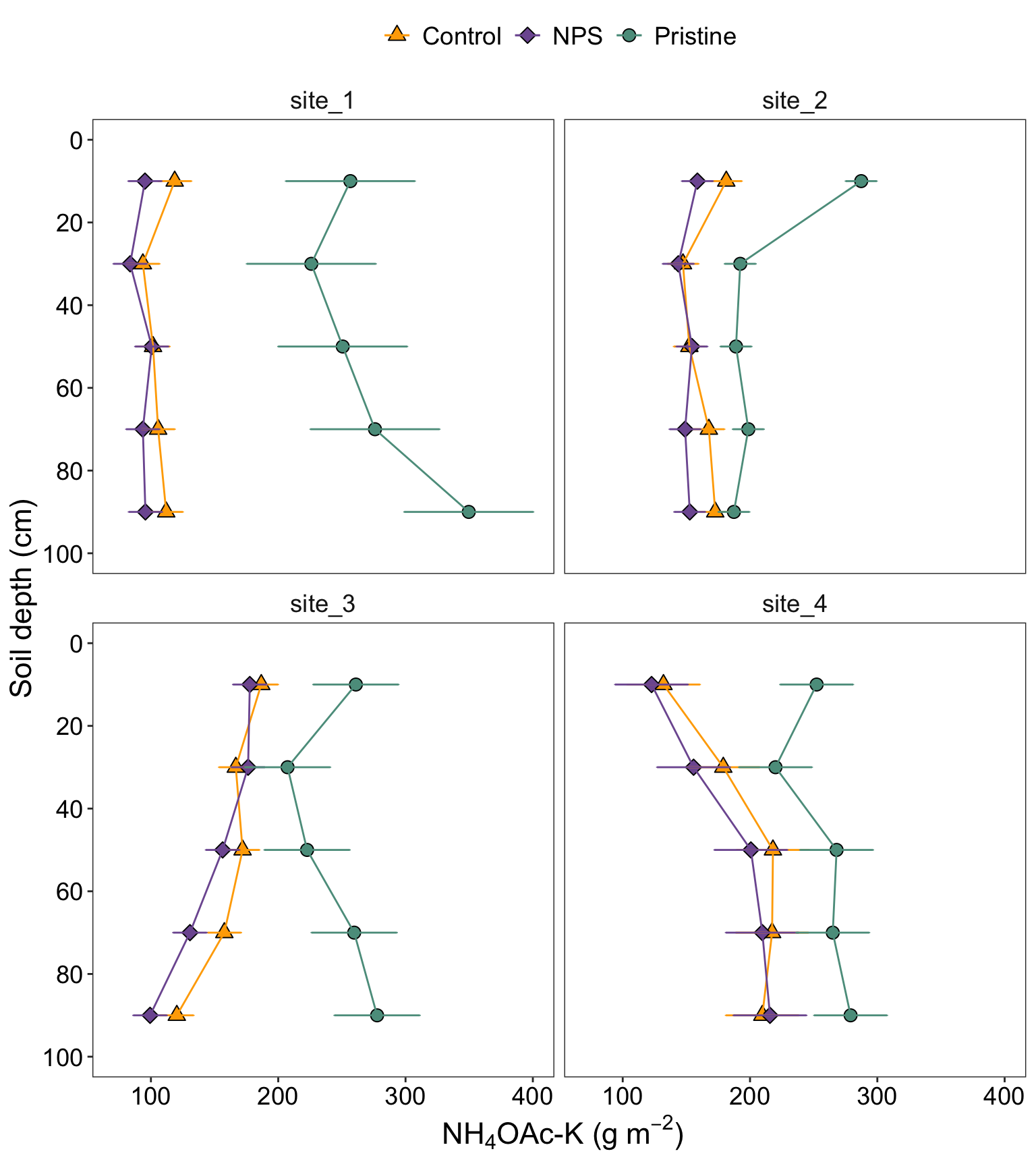
2.6.1 Figure with caption
STK_plot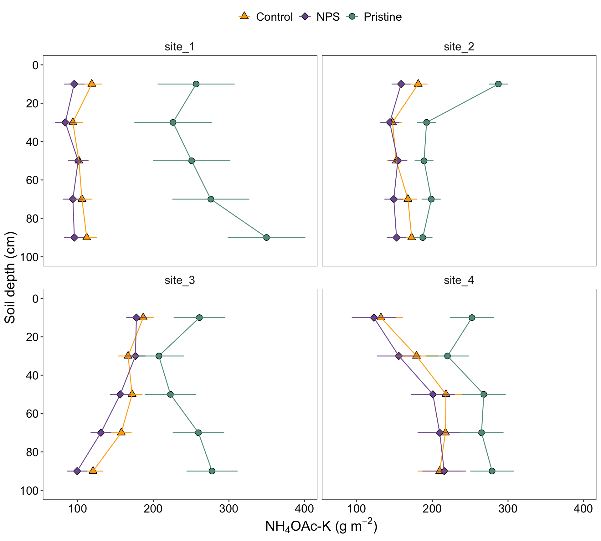
Figure 2. Soil profiles of STK (\(g~m^{-2}\)) under three different conditions: pristine soils (green circles), under grain cropping from 2000 to 2009 with no fertilizers added (Control, orange triangles), and under grain cropping from 2000 to 2009 with N, P, plus S fertilization (NPS, purple diamonds). Overlapping error bars indicate absence of significant differences between scenarios by soil depths combinations (0.05).
References
Correndo, Adrian A., Gerardo Rubio, Fernando O. García, and Ignacio A. Ciampitti. 2021. “Subsoil-Potassium Depletion Accounts for the Nutrient Budget in High-Potassium Agricultural Soils.” Scientific Reports 11 (1). https://doi.org/10.1038/s41598-021-90297-1.
Dixon, Philip. 2016. “Should Blocks Be Fixed or Random?” Conference on Applied Statistics in Agriculture, May 1-3, Kansas State University, 23–39. https://doi.org/10.4148/2475-7772.1474.
Zuur, Alain F., Elena N. Ieno, and Chris S. Elphick. 2010. “A Protocol for Data Exploration to Avoid Common Statistical Problems.” Methods in Ecology and Evolution 1 (1): 3–14. https://doi.org/https://doi.org/10.1111/j.2041-210X.2009.00001.x.